Study Plan

The order in which to read the orbital mechanics notes

Read the notes in the order given below: each one uses only what came before it. The plan is for students of AE313/AE613 who know school physics, first-year calculus and vectors, and nothing about orbits.

How to use this plan

What to expect in a note:

• An opening section that lists the questions you will be able to answer by the end. Read it first, and come back to it at the end to check yourself.
• Derivations in full. Work through them with a pen; do not just read them.
• Try it / Check yourself boxes in many notes. Stop and do them before reading on.
• Margin boxes on history. Enjoy them, but you can skip them on a first reading.
• Scripts. Every figure links to the script that drew it, and the numbers in each note are checked by a verify script in the codes folder. Run them if you want to experiment.
• One set of symbols. The notation page lists the symbols and the constants that all the notes share.

How to study one note:

1. Read the opening questions and the summary at the end (about 10 minutes).
2. Read the note straight through, redoing each derivation on paper.
3. Do every Try it box, then the problems listed for that stage in this plan.
4. Before moving on, answer the opening questions out loud, without looking.

The reading order

There are 18 steps in seven stages, about 57 hours of reading before the problem sets. Each note uses only the notes above it, except where a row says a part can wait. Level runs from 1 (gentle) to 5 (hard). Stages 1 to 4 are the core of AE313; stages 5 to 7 complete AE613 and the full picture.

Stage 1: Foundations (about 10 hours)

Step	Note	Read after	After it you can	Time	Level
1	The N-Body Problem	School physics, vectors, first-year calculus	Write the equations of motion, derive the ten integrals, and explain why spaceflight uses one attracting body at a time	2–2.5 h	2
2	The Two-Body Problem	Step 1	Get \(\mathbf h\), \(\mathbf e\), energy, \(a\), \(p\) and the conic from a state; speeds, flight-path angle and escape; Kepler’s equation for all three conics; a flyby’s turning angle	5 h	3
3	Tutorial 1	Step 2	Run the whole state-to-orbit chain on real problems and decide whether an orbit hits the Earth	2–2.5 h	2

The two-body note is long. On a first pass, read Part 1 (“What every orbit shares”) and the ellipse up to Kepler’s equation. Come back for the parabola and the hyperbola before stage 4.

Stage 2: Orbits in three dimensions (about 7 hours)

Step	Note	Read after	After it you can	Time	Level
4	The Perifocal Frame	Step 2	Build the orbit’s own axes from \(\mathbf h\) and \(\mathbf e\), write position and velocity in them, and rotate them into space	2–2.5 h	3
5	Orbital Elements	Step 4	Convert a state to the six elements and back with quadrant-safe formulas, handle circular and equatorial orbits, and design a sun-synchronous inclination	2.5–3 h	3
6	Time	Step 5	Tell the sidereal day from the solar day, move between UT1, UTC, TAI, TT and TDB, compute Julian dates and sidereal time, and turn a clock error into a position error	2 h	3

Stage 3: Manoeuvres (about 5 hours)

Step	Note	Read after	After it you can	Time	Level
7	Orbital Manoeuvres	Steps 2 and 5	Cost and time a Hohmann, bi-elliptic, phasing, apse-rotation, plane-change and escape manoeuvre; explain the Oberth effect; turn \(\Delta v\) into propellant	4–5 h	3

The two proofs (aligned apsides, Hohmann optimality) can wait for a second reading.

Stage 4: Going to other worlds (about 5 hours)

Step	Note	Read after	After it you can	Time	Level
8	Patched Conics	Steps 2 (hyperbola) and 7 (Hohmann)	Derive the sphere of influence, plan an Earth–Mars transfer conic by conic, choose where to burn, size a flyby, and handle out-of-plane departures and arrivals	4–5 h	3.5

Stage 5: Targeting and rendezvous (about 13 hours)

Step	Note	Read after	After it you can	Time	Level
9	Lambert’s Problem	Steps 4 and 7	Find the conic through two points in a given time, both ways round and with several revolutions, and know where the solver struggles	4 h	4
10	Universal Variables	Steps 8 and 9	Propagate any orbit with one equation and no case split, and solve Lambert’s problem in the universal variable	3 h	4
11	Relative Motion and the CW Equations	Step 2; step 9 for motivation	Derive and solve the Clohessy–Wiltshire equations, predict drift and fly-arounds, and use the state-transition matrix	3–3.5 h	3.5
12	Chase Manoeuvres	Steps 7, 9 and 11	Design phasing orbits, read a porkchop plot, pick intercept or rendezvous optima, and target the final approach	3 h	3

Stage 6: The real Earth (about 10 hours)

Step	Note	Read after	After it you can	Time	Level
13	Beyond the Point Mass, up to “The \(J_2\) potential and acceleration”	Step 1	Expand the Earth’s potential in Legendre functions, read the coefficient table, and compute the \(J_2\) acceleration	2 h	4
14	Deriving the Gauss Variational Equations	Steps 5 and 11	Derive how any small force changes each element, and see which burn direction moves which element, and where	3–4 h	4
15	Beyond the Point Mass, from “What \(J_2\) does to an orbit” to the end	Steps 13 and 14	Derive and use the nodal regression and apsidal rotation, design sun-synchronous and frozen orbits, and explain geostationary drift	2–3 h	4
16	Ground Tracks	Steps 6 and 15	Compute a ground track from the elements, and design repeat, sun-synchronous and Molniya tracks, footprints and launch azimuths	2–3 h	3

Stage 7: The sky and the third body (about 7 hours)

Step	Note	Read after	After it you can	Time	Level
17	Topocentric Frames and Observations	Steps 5, 6 and 16	Put a station on the reference ellipsoid, build its south-east-zenith frame, convert a state to azimuth, elevation, range and their rates (and back), relate right ascension and declination to them, and say what limits each measurement	3 h	3
18	The Circular Restricted Three-Body Problem	Steps 1, 8 and 11	Write the restricted problem in the rotating frame, use the Jacobi constant to draw forbidden regions, find and test the five Lagrange points, and describe halo orbits	4 h	4

Step 17 is the doorway to orbit determination (Gibbs, Lambert-based and angles-only methods), which the notes do not yet cover. Step 18 can be read as soon as steps 8 and 11 are done; it uses the rotating-frame kinematics of the CW note and the sphere of influence of the patched-conics note.

Optional enrichment

• Advanced Manoeuvres, after step 9: optimal single-impulse intercepts, deorbit burns and escape to a given \(v_\infty\), and the Hohmann cost over four decades of radius ratio. About 2.5 h, level 4. Part III (escape) can be read straight after step 7, as a companion to its escape section.

How the notes depend on each other

Figure 1: An arrow means “read this first”. The numbers are the steps of the reading order. Script: fig-study-plan.py.

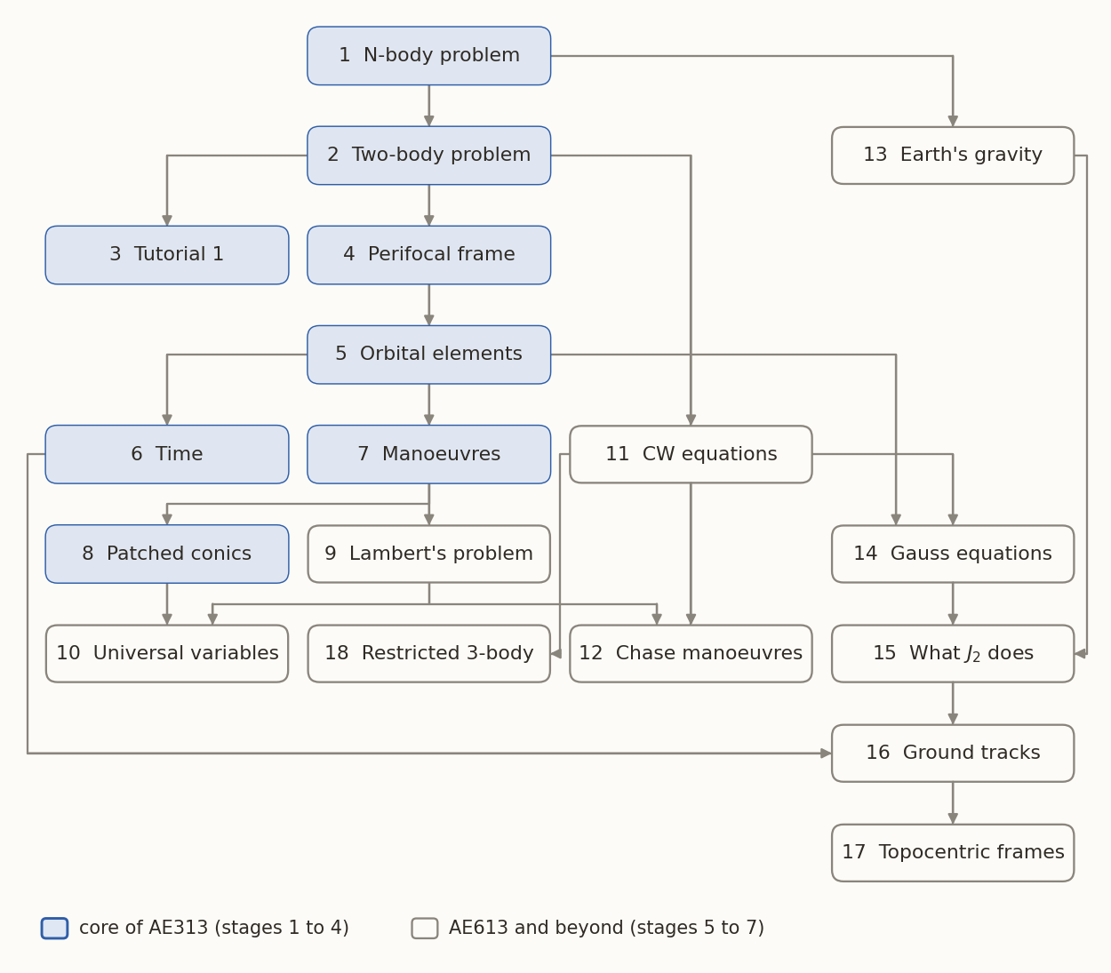
Two branches can be read in either order once their arrows are satisfied: the CW equations (11) need only the two-body note, and the potential half of Earth’s gravity (13) needs only the N-body note. The restricted three-body problem (18) is drawn with an arrow from the CW equations (11); it also uses the patched-conics note (8), which the figure leaves out to keep the lines apart.

In a hurry (an exam in a week): steps 1, 2 (Part 1 and Kepler’s equation), 4, 5, 7 and 8, with Tutorial 1 and the objective questions for those topics. That is about 20 hours, and it covers the AE313 syllabus except ground tracks and topocentric frames.

Problems: when to attempt each set

Do the problems straight after the step named. A set attempted too early sends you to material you have not met; one left too late stops being practice.

Set	Attempt after	What it trains	Time	Level
Tutorial 1	Step 2 (it is step 3)	The state-to-orbit chain on real cases	2–2.5 h	2
Objective questions, N-body (Q1–50)	Step 1; Q36 after step 2, Q41 and Q49 after step 8	Quick checks of the ideas	about 2.5 h	1–4
Objective questions, two-body (Q51–100)	Step 2; Q90 after Tutorial 1	The same, for conics, energy and Kepler’s equation	about 2.5 h	1–4
Objective questions, elements (Q101–150)	Step 5; Q117, Q118, Q143 need step 4; Q125, Q126, Q134, Q137 need step 16; Q147 needs step 14	The same, for frames and elements	about 2.5 h	1–4
Objective questions, manoeuvres (Q151–200)	Step 7; Q176–177 after step 8; Q184 and Q200 after step 9; Q199 after step 11	The same, for manoeuvres	about 2.5 h	1–4
Orbital Maneuvers: Analytical Problems	Step 7	Turning a cost into a formula, and proving optima and thresholds	5–6 h	4
Orbital Elements: Analytical Problems	Step 7 (it refers back to the manoeuvres note); P10 after step 15	Reasoning about elements without numbers: symmetries, degenerate cases, impulse sensitivities	4–5 h	4
Orbital Maneuvers: Problems, Q1–Q4	Step 7	How execution errors in magnitude, pointing and timing spread through a manoeuvre	3 h	3
Orbital Maneuvers: Problems, Q5–Q10	Step 8	Sizing real burns and propellant; when the impulsive model fails	4–5 h	3–4
Indian Missions: Trajectory Problems, Problems 1–5	Steps 8 and 9	Rebuilding Chandrayaan, Mangalyaan and Aditya-L1 \(\Delta v\) budgets from published orbits	3–3.5 h	3
Indian Missions, Problem 6	Step 18	L1 and halo-orbit basics: the Jacobi constant, the neck at \(L_1\), the stable manifold and the price of a short cruise	1.5 h	4.5

In the objective questions, Level 1 takes about a minute a question, Level 2 about three and Level 3 six to eight. Do Level 1 the day you finish a note, and Level 3 a week later as revision.

The exercises at the end of each note are not repeated here: do them before moving to the next step.