Beyond the Point Mass

The Earth’s gravity field, where its harmonics come from, and what they do to an orbit

1 Where we are going

Up to now the Earth has been a point mass: every satellite obeys \[ \ddot{\mathbf r} = -\frac{\mu}{r^{3}}\,\mathbf r ,\qquad \mu = GM_\oplus , \] and the orbit is a fixed conic in inertial space forever. Real satellites disagree. The orbital plane of the International Space Station turns about the Earth’s axis by roughly \(5^\circ\) every day; the plane of a Sun-synchronous imaging satellite turns by exactly \(0.9856^\circ\) per day so that it keeps a constant angle to the Sun; a geostationary satellite parked over the Indian Ocean slowly slides along the equator unless it is nudged back. None of this is possible under \(-\mu\mathbf r/r^3\).

The cause is that the Earth is not a sphere. It spins, so it bulges at the equator (the equatorial radius exceeds the polar radius by about \(21\) km), and its interior is lumpy. Figure 1 shows the idea.

Figure 1: Left: the Earth’s cross-section with the flattening exaggerated \(36\) times. The bulge pulls a satellite slightly toward the equatorial plane, in addition to the usual pull towards the centre. Right: a useful mental model, which we will make quantitative: an oblate Earth is a sphere with a belt of extra mass added at the equator and mass removed from the polar caps. Script: fig-grav-basics.py.

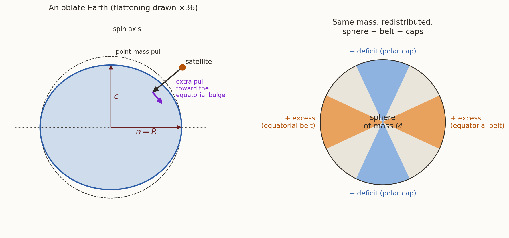
History. Newton’s Principia (1687) already argued that a spinning Earth must flatten at the poles, and estimated the flattening at about \(1/230\). Cassini’s meridian measurements in France seemed to say the opposite (a prolate Earth). The dispute was settled by the French geodesic expeditions to Lapland (Maupertuis, Clairaut, Celsius, 1736–37) and to Peru (Bouguer, La Condamine, Godin, 1735–44): degrees of latitude are longer near the poles, so the Earth is oblate. Clairaut’s Théorie de la figure de la Terre (1743) turned this into mathematics.

The aim of this note is to replace the point-mass law by a systematic, improvable description of the Earth’s gravity, and to understand its consequences. When you finish, you should be able to answer, without hand-waving, all of the following.

1. Why do we describe gravity by a scalar potential rather than by the force vector?
2. Why is the potential expanded in Legendre polynomials, and where do they come from?
3. What are the numbers \(J_2, J_3, C_{22}, S_{22},\dots\) physically, in terms of the Earth’s mass distribution?
4. Why is the same list of functions guaranteed to be complete (Laplace’s equation, separation of variables)?
5. How do we get from the \(J_2\) potential to an explicit acceleration vector?
6. How does the \(J_2\) acceleration make an orbit’s plane precess, and why is there a “critical inclination”?
7. How does the next harmonic, \(C_{22}/S_{22}\), explain the drift of geostationary satellites?

What you need to know, and what you don’t

You need: the gradient of a scalar function, the chain rule for partial derivatives, the binomial series \((1+u)^{-1/2}\), and how to solve an ODE by a power series. You do not need Bessel functions, special-function tables or any prior contact with Legendre polynomials or spherical harmonics. Each tool is introduced at the moment it is needed, together with a box explaining why this tool and not another.

2 Conventions used throughout

Table 1: Notation

Symbol	Meaning
\(\mu = GM_\oplus\)	Earth’s gravitational parameter, \(398\,600.44\ \text{km}^3/\text{s}^2\)
\(R\)	Earth’s equatorial radius, \(6378.137\) km (a reference length; it just makes coefficients dimensionless)
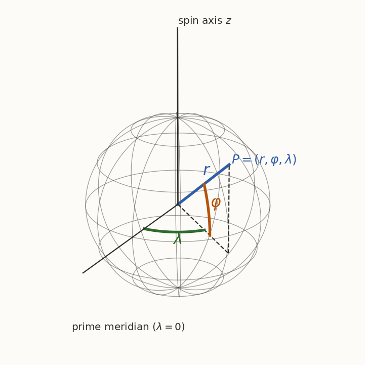
\((r,\varphi,\lambda)\)	Radius, geocentric latitude (positive north), east longitude, all in the Earth-fixed frame
\(\mathbf r,\ \mathbf r'\)	Position of the field point \(P\) (where we want gravity) and of a mass element \(dm'\)
\(U\)	Gravitational potential, defined with the sign such that \(\mathbf a=+\nabla U\)
\(\mathcal R\)	The perturbing (disturbing) part of \(U\): \(U=\mu/r+\mathcal R\)
\(x=\sin\varphi\) or \(\cos\gamma\)	Argument of the Legendre functions

Latitude caveat. \(\varphi\) here is the geocentric latitude (angle from the equatorial plane to the position vector). The geodetic latitude on maps and GPS receivers differs by up to \(0.19^\circ\). The harmonic expansions are naturally written in geocentric latitude.

3 From force to potential

3.1 One scalar instead of three vectors

For a point mass at the origin, define \[ U(\mathbf r) = \frac{\mu}{r}, \qquad r=\sqrt{x^2+y^2+z^2}. \] Its gradient is computed with \(\partial r/\partial x = x/r\): \[ \frac{\partial U}{\partial x} = -\frac{\mu}{r^{2}}\frac{\partial r}{\partial x}= -\frac{\mu x}{r^{3}} \quad\Longrightarrow\quad \nabla U = -\frac{\mu}{r^{3}}\,\mathbf r = \ddot{\mathbf r}. \] So the acceleration is the gradient of a single scalar function. We call \(U\) the potential.¹

¹ Physics texts define the potential energy per unit mass as \(-\mu/r\) and then write \(\mathbf a=-\nabla(\text{energy})\). Geodesy and astrodynamics drop the minus sign so that \(U>0\) and \(\mathbf a=+\nabla U\). Both conventions describe the same physics. We use the second, because it makes the series in Section 4 come out with plus signs.

History. Lagrange (1773) noticed that the gravitational force of any mass distribution is the gradient of one scalar function. The name “potential” was coined by George Green (1828, a self-taught Nottingham miller) and independently by Gauss (1839–40), who built the whole theory of harmonic functions on it.

3.2 Extended bodies: add scalars, not vectors

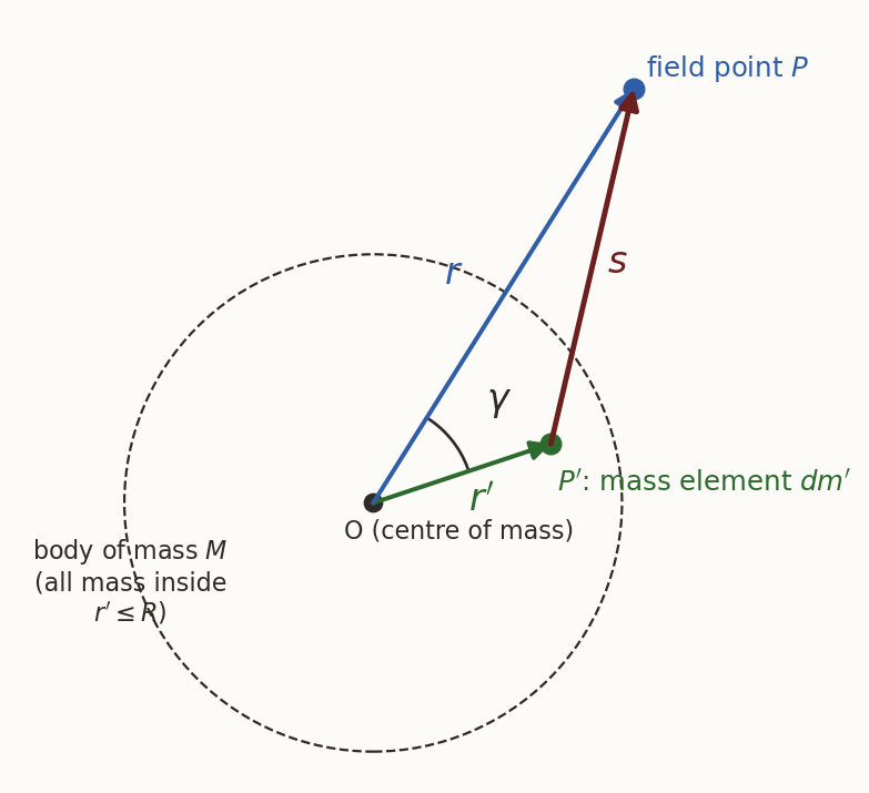
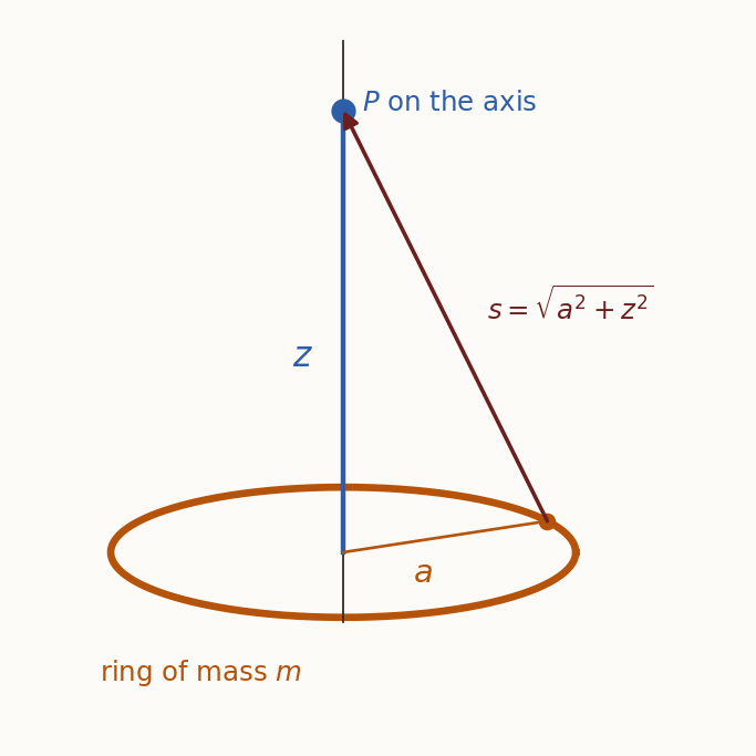
Now let the Earth consist of many small mass elements \(dm'\) at positions \(\mathbf r'\). The field point is \(P\) at \(\mathbf r\), and the separation is \(s=|\mathbf r-\mathbf r'|\) (Figure 2). Newton’s law says each element pulls with acceleration \(G\,dm'/s^{2}\) along the line to it, so we must add vectors that all point in different directions. Instead, add the scalar potentials, which are just numbers: \[ U(P) = G\int_{\text{Earth}} \frac{dm'}{s}, \qquad s=|\mathbf r-\mathbf r'| . \tag{1}\]

Figure 2: Geometry for the potential of one mass element. \(O\) is the centre of mass. The mass element sits at \(P'\) (position \(\mathbf r'\)). Every element has \(r'\le R\), and we evaluate the field at a point \(P\) with \(r>R\). The angle \(\gamma\) between \(\mathbf r\) and \(\mathbf r'\) will be the key variable. Script: fig-grav-basics.py.

That this is the right thing follows because \(\nabla\) acts only on the field point \(\mathbf r\) and passes inside the integral: \[ \nabla U = G\int \nabla\!\left(\frac1s\right)dm' = -G\int \frac{\mathbf r-\mathbf r'}{s^{3}}\,dm' , \] which is exactly the vector sum of all the Newtonian pulls. One scalar integral has done the work of three vector ones.

The real difficulty, and the plan

Equation 1 is exact but useless as it stands: to evaluate it we would need the density of the Earth at every interior point, which nobody knows. The plan is therefore:

1. Expand \(1/s\) so that the dependence on the field point (\(r,\varphi,\lambda\)) is separated from the dependence on the mass element (\(r',\varphi',\lambda'\)).
2. What remains of the mass distribution is a list of numbers (integrals of \(dm'\) times simple functions, called moments).
3. We never compute these moments from a density model. We measure them from the orbits of satellites. The list of numbers is the gravity model.

4 Expanding \(1/s\): the origin of the Legendre polynomials

4.1 Step 1: law of cosines

In the triangle \(O\)–\(P'\)–\(P\) of Figure 2, \[ s^2 = r^2 + r'^2 - 2rr'\cos\gamma . \] Factor out \(r^2\) and introduce the two dimensionless quantities \[ \varepsilon \equiv \frac{r'}{r}, \qquad x\equiv\cos\gamma , \] to obtain \[ \frac1s = \frac1r\,\bigl(1-2x\varepsilon+\varepsilon^2\bigr)^{-1/2}. \tag{2}\]

Why expand in \(\varepsilon\)? Because when \(P\) lies outside the body, \(r'<r\) for every mass element, so \(\varepsilon<1\): a natural small parameter. And powers of \(\varepsilon\) automatically separate the two positions, since \(\varepsilon^n = r'^{\,n}/r^{n}\): the mass element appears only in the numerator, the field point only in the denominator.

4.2 Step 2: binomial series, term by term

Write \(u=-2x\varepsilon+\varepsilon^2\) and use \((1+u)^{-1/2}=1-\tfrac12u+\tfrac38u^2-\tfrac5{16}u^3+\cdots\). Collect powers of \(\varepsilon\), being careful that \(u\) itself contains \(\varepsilon\) and \(\varepsilon^2\):

\[ \begin{aligned} -\tfrac12 u &= x\,\varepsilon-\tfrac12\varepsilon^2,\\[2pt] +\tfrac38 u^2 &= \tfrac38\left(4x^2\varepsilon^2-4x\varepsilon^3+\varepsilon^4\right)=\tfrac32x^2\varepsilon^2-\tfrac32x\varepsilon^3+\cdots,\\[2pt] -\tfrac5{16}u^3 &= -\tfrac5{16}\left(-8x^3\varepsilon^3+\cdots\right)=\tfrac52x^3\varepsilon^3+\cdots . \end{aligned} \] Adding up, by powers of \(\varepsilon\):

Table 2: The first coefficients of the expansion of \((1-2x\varepsilon+\varepsilon^2)^{-1/2}\).

power	coefficient
\(\varepsilon^0\)	\(1\)
\(\varepsilon^1\)	\(x\)
\(\varepsilon^2\)	\(-\tfrac12+\tfrac32x^2=\tfrac12(3x^2-1)\)
\(\varepsilon^3\)	\(-\tfrac32x+\tfrac52x^3=\tfrac12(5x^3-3x)\)

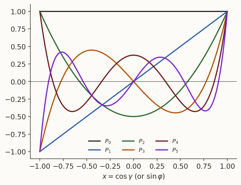
Definition. The coefficient of \(\varepsilon^n\) is called the Legendre polynomial \(P_n(x)\): \[ \boxed{\ \frac{1}{\sqrt{1-2x\varepsilon+\varepsilon^{2}}}=\sum_{n=0}^{\infty}P_n(x)\,\varepsilon^{n}\ } \tag{3}\] Thus \(P_0=1\), \(P_1=x\), \(P_2=\tfrac12(3x^2-1)\), \(P_3=\tfrac12(5x^3-3x)\). It is not a new function invented for convenience: it is the \(n\)th Taylor coefficient of \(1/s\), in the variable \(\varepsilon\). Note the subtlety: a Taylor coefficient of a function of one variable is a number, but here the function \((1-2x\varepsilon+\varepsilon^2)^{-1/2}\) also depends on the parameter \(x=\cos\gamma\). We expand in \(\varepsilon\) for each fixed \(x\), so the coefficient of \(\varepsilon^n\) is a number for that \(x\), and a function \(P_n(x)\) as \(x\) varies. Section 13 makes this precise.

History. Adrien-Marie Legendre introduced these polynomials in 1782 in a memoir on the attraction of spheroids, in exactly this way: expanding the Newtonian potential \(1/s\). Laplace, who was working on the same problem for the shape of the planets, used and named them within the same few years.

Figure 3: The first six Legendre polynomials. \(P_n\) has \(n\) zeros in \((-1,1)\), all of them “wiggles” of magnitude at most \(1\). Every \(P_n(1)=1\). Script: fig-grav-basics.py.

4.3 Step 3: a recurrence, and two facts we will use

Higher polynomials need not be found by grinding through the binomial series. Differentiate Equation 3 with respect to \(\varepsilon\) and multiply by \((1-2x\varepsilon+\varepsilon^2)\); the left side becomes \((x-\varepsilon)(1-2x\varepsilon+\varepsilon^2)^{-1/2}\), so \[ (1-2x\varepsilon+\varepsilon^2)\sum_n nP_n\varepsilon^{n-1}=(x-\varepsilon)\sum_nP_n\varepsilon^n . \] The coefficient of \(\varepsilon^n\) on each side is \[ (n+1)P_{n+1}-2xnP_n+(n-1)P_{n-1}=xP_n-P_{n-1} \ \Longrightarrow\ \boxed{(n+1)P_{n+1}=(2n+1)\,x\,P_n-nP_{n-1}} \tag{4}\] For instance \(4P_4=7xP_3-3P_2=\tfrac12(35x^4-30x^2+3)\), so \(P_4=\tfrac18(35x^4-30x^2+3)\).

Two facts follow directly from Equation 3:

• \(P_n(1)=1\). At \(x=1\) (\(\gamma=0\), the two positions on the same ray) the left side is \(1/(1-\varepsilon)=\sum\varepsilon^n\).
• \(P_n(0)\): e.g. \(P_2(0)=-\tfrac12\), \(P_4(0)=\tfrac38\) (we use these below).

4.4 Step 4: does it converge, and how fast?

Why the series converges (and why we may keep only a few terms)

Factorise the quantity under the root: \(1-2x\varepsilon+\varepsilon^2=(1-\varepsilon e^{i\gamma})(1-\varepsilon e^{-i\gamma})\) (multiply out and use \(2\cos\gamma=e^{i\gamma}+e^{-i\gamma}\)). Each factor has its own binomial series, \[ (1-\varepsilon e^{\pm i\gamma})^{-1/2}=\sum_{k\ge0}c_k\,\varepsilon^{k}e^{\pm ik\gamma},\qquad c_k=\binom{2k}{k}4^{-k}>0 . \] Multiplying the two series and collecting \(\varepsilon^n\) gives \[ P_n(\cos\gamma)=\sum_{k=0}^{n}c_kc_{n-k}\cos\bigl((n-2k)\gamma\bigr). \] (Check for \(n=2\): \(c_0=1,\ c_1=\tfrac12,\ c_2=\tfrac38\) give \(\tfrac34\cos2\gamma+\tfrac14=\tfrac12(3\cos^2\gamma-1)\). ✓.) Since \(|\cos|\le1\), \(|P_n(\cos\gamma)|\le\sum c_kc_{n-k}=P_n(1)=1\). Therefore each term of Equation 3 obeys \(|P_n(x)\,\varepsilon^n|\le\varepsilon^n\). This is a term-by-term bound (comparison test): the series is dominated by the geometric series \(\sum\varepsilon^n=1/(1-\varepsilon)\), which converges for \(\varepsilon<1\), so Equation 3 converges too. The expansion works when the field point is outside the sphere that contains all the mass (\(r>R\)). Because \(|P_n|\le1\), the tail after the term \(n=N\) is at most \(\varepsilon^{N+1}/(1-\varepsilon)\).

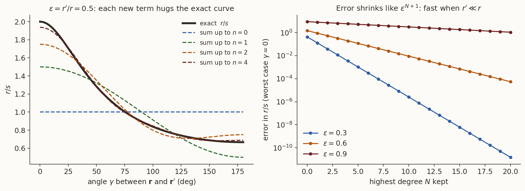
Figure 4 shows this. The left panel shows the partial sums hugging the exact \(r/s\) as more terms are added. The right panel shows the error for the worst case \(\gamma=0\): it falls like \(\varepsilon^{N+1}\). A satellite at \(r=7000\) km sees mass elements at \(r'\le6378\) km, so \(\varepsilon\le0.91\) for the very outermost mass, but for the bulk of the Earth’s mass \(\varepsilon\) is much smaller, which is why the low terms carry nearly all the information.

Figure 4: Left: exact \(r/s\) for \(\varepsilon=0.5\) versus partial sums of Equation 3. Right: the error of the partial sum at \(\gamma=0\) (the slowest case). Small \(\varepsilon\) (mass far below the field point) needs few terms; \(\varepsilon\to1\) (skimming the surface) needs many. Script: fig-grav-basics.py.

4.5 Step 5: the potential as a series of multipoles

Insert Equation 3 into Equation 1 with \(\varepsilon=r'/r\). Since only \(r'\), \(\gamma\), \(dm'\) depend on the mass element, \(1/r^{n+1}\) leaves the integral: \[ \boxed{\ U(P)=\sum_{n=0}^{\infty}\frac{G}{r^{n+1}}\int r'^{\,n}\,P_n(\cos\gamma)\,dm'\ } \tag{5}\] Look at what has happened: the \(n\)th term falls off like \(r^{-(n+1)}\), so higher terms die faster with distance, and each is multiplied by a “moment” of the mass distribution. This is precisely the step that separated what we know (geometry of \(P\)) from what we measure (the moments). The first few terms have simple meanings.

• \(n=0\) (monopole). \(P_0=1\): \(\;U_0=\dfrac{G}{r}\int dm'=\dfrac{GM}{r}=\dfrac{\mu}{r}\). This is the point-mass term we have been using.
• \(n=1\) (dipole). \(P_1=\cos\gamma\), and \(r'\cos\gamma=\hat{\mathbf r}\cdot\mathbf r'\), so \(U_1=\dfrac{G}{r^{2}}\,\hat{\mathbf r}\cdot\int\mathbf r'\,dm'=\dfrac{GM}{r^{2}}\,\hat{\mathbf r}\cdot\mathbf r_{\rm cm}\). It vanishes when the origin is the centre of mass, which is why we always place it there: no first-degree term exists in any Earth-centred gravity model.
• \(n=2\) (quadrupole). The first term that can distinguish an oblate body from a sphere. We evaluate it in Section 4.6.

Degree n = 2 (quadrupole) Cut-away

Figure 5: Interactive. Move the slider to choose \(n\); drag to rotate, scroll to zoom, and use the toolbar (top right of the plot) to switch to pan. Each surface is a surface of revolution about the axis \(\mathbf r'\) points along (tick Cut-away to remove a quarter and show the inside); its radius in direction \(\gamma\) from that axis is \(|P_n(\cos\gamma)|\). Blue lobes are positive, red lobes negative. This is not a picture of a body. It plots the angular pattern of the function \(P_n(\cos\gamma)\): the distance from the origin in each direction is the value of \(|P_n|\) there, so the monopole (\(P_0=1\)) is just a unit-radius surface (a sphere, drawn hollow), not a solid ball or a shell of mass. How it was made: the page evaluates \(P_n\) with Equation 4 on a grid of \(\gamma\in[0,\pi]\) and azimuth (longitude-like angle) \(\lambda\), sets \(\rho=|P_n(\cos\gamma)|\), maps to \((x,y,z)=\rho\,(\sin\gamma\cos\lambda,\ \sin\gamma\sin\lambda,\ \cos\gamma)\), colours each point by the sign of \(P_n\), and draws it with Plotly.js. The code is the inline JavaScript of this page (view source); a static matplotlib version is in fig-grav-basics.py. The monopole is isotropic; the dipole has a positive and a negative hemisphere; each higher \(n\) adds one more sign change. A real mass distribution is a weighted sum of such patterns.

Sanity check 1: a sphere is a point mass (Newton’s shell theorem)

If the Earth were spherically symmetric, for every mass element at \(\mathbf r'\) there would be others at the same \(r'\) in all directions, so for \(n\ge1\) the integral in Equation 5 reduces to \(\int P_n(\cos\gamma)\,d(\text{solid angle})\propto\int_{-1}^{1}P_n(x)\,dx\). This vanishes for \(n\ge1\) (for instance \(\int_{-1}^1x\,dx=0\) and \(\int_{-1}^1\tfrac12(3x^2-1)\,dx=0\)). Only the monopole survives, and the sphere attracts exactly like a point mass. Every departure from the point-mass law is therefore a measure of departure from spherical symmetry.

Sanity check 2: a ring on its axis

Take a ring of mass \(m\) and radius \(a\) in the equatorial plane, and a field point on the axis at height \(z\) (Figure 6). Then every ring element has \(\gamma=90^\circ\), \(r'=a\), \(r=z\). Equation 5 gives immediately \[ U=\frac{Gm}{z}\sum_n P_n(0)\left(\frac{a}{z}\right)^{n}=\frac{Gm}{z}\left(1-\tfrac12\frac{a^2}{z^2}+\tfrac38\frac{a^4}{z^4}-\cdots\right). \] Directly: \(U=Gm/\sqrt{a^2+z^2}=\frac{Gm}{z}\bigl(1+a^2/z^2\bigr)^{-1/2}=\frac{Gm}{z}\bigl(1-\tfrac12a^2/z^2+\tfrac38a^4/z^4-\cdots\bigr)\). ✓ Note the sign of the \(n=2\) term: a belt of mass at the equator reduces the potential on the polar axis below \(\mu/z\), because that mass is farther from the pole than it would be if it were concentrated at the centre. Keep this in mind: it is the origin of the minus sign in front of \(J_2\) later.

Figure 6: A ring of mass at the equator, evaluated on the axis. All ring elements have \(\gamma=90^\circ\). Script: fig-grav-basics.py.

4.6 The quadrupole term and MacCullagh’s formula

For \(n=2\), \(P_2(\cos\gamma)=\tfrac12(3\cos^2\gamma-1)\), so \[ U_2=\frac{G}{2r^{3}}\int r'^{2}\bigl(3\cos^2\gamma-1\bigr)dm' . \] Let \(I\) be the moment of inertia of the body about the line \(OP\). The distance of \(dm'\) from that line is \(r'\sin\gamma\), so \(I=\int r'^2\sin^2\gamma\,dm'\), i.e. \(\int r'^2\cos^2\gamma\,dm'=\int r'^2dm'-I\). With the principal moments \(A,B,C\) (about \(x,y,z\); note \(A+B+C=2\int r'^2dm'\)), \[ U_2=\frac{G}{2r^3}\Bigl[3\!\int r'^2dm'-3I-\!\int r'^2dm'\Bigr]=\frac{G}{2r^{3}}\Bigl[\,A+B+C-3I\,\Bigr]. \tag{6}\] This is MacCullagh’s formula. It says the leading correction to \(\mu/r\) depends on the body only through its moments of inertia, quantities we associate with rotational dynamics, not with any detailed density map.

History. James MacCullagh (Dublin, 1840) found this compact formula for the first correction to the attraction of any body. Today the moments of inertia (\(A,B,C\)) of the Earth are among the best determined numbers in geophysics, obtained from the precession of the equinoxes and from satellite orbits.

5 Latitude and longitude: the addition theorem

Equation 5 is in terms of the angle \(\gamma\) between \(P\) and \(dm'\). But the Earth’s mass distribution is fixed in the rotating, Earth-fixed frame, where each mass element has a definite latitude \(\varphi'\) and longitude \(\lambda'\), and we want gravity at a definite \((\varphi,\lambda)\). So we need \(\cos\gamma\) in terms of these angles.

Figure 7: Geocentric spherical coordinates. \(\varphi\) is measured from the equatorial plane (north positive), \(\lambda\) eastward from the prime meridian. Script: fig-grav-harmonics.py.

5.1 The angle between two directions

Unit vectors in these coordinates are \(\hat{\mathbf r}=(\cos\varphi\cos\lambda,\ \cos\varphi\sin\lambda,\ \sin\varphi)\) and similarly for \(\hat{\mathbf r}'\). Their dot product is \(\cos\gamma\): \[ \cos\gamma=\sin\varphi\sin\varphi'+\cos\varphi\cos\varphi'\cos(\lambda-\lambda'). \tag{7}\] Note that longitude enters only through the difference \(\Delta\equiv\lambda-\lambda'\).

5.2 \(n=1\) and \(n=2\) done by hand

Write \(s_\varphi=\sin\varphi,\ c_\varphi=\cos\varphi\) (and primes for the mass element). For \(n=1\), \(P_1(\cos\gamma)=\cos\gamma\) is Equation 7 itself. For \(n=2\) square Equation 7 and use \(\cos^2\Delta=\tfrac12(1+\cos2\Delta)\): \[ \cos^2\gamma=s_\varphi^2s_{\varphi'}^2+2s_\varphi s_{\varphi'}c_\varphi c_{\varphi'}\cos\Delta+\tfrac12c_\varphi^2c_{\varphi'}^2\,(1+\cos2\Delta). \] Then \[ P_2(\cos\gamma)=\underbrace{\tfrac12\Bigl[3s_\varphi^2s_{\varphi'}^2+\tfrac32c_\varphi^2c_{\varphi'}^2-1\Bigr]}_{(\mathrm{i})} +\underbrace{3\,s_\varphi c_\varphi\,s_{\varphi'}c_{\varphi'}\cos\Delta}_{(\mathrm{ii})} +\underbrace{\tfrac34\,c_\varphi^2c_{\varphi'}^2\cos2\Delta}_{(\mathrm{iii})}. \] Now the miracle: each piece factorises into a function of \(\varphi\) times the same function of \(\varphi'\).

• (i): put \(S=s_\varphi^2,\ S'=s_{\varphi'}^2\) and \(c^2=1-S\). Then \(3SS'+\tfrac32(1-S)(1-S')-1=\tfrac92SS'-\tfrac32S-\tfrac32S'+\tfrac12\), so (i)\(=\tfrac14(9SS'-3S-3S'+1)=\tfrac14(3S-1)(3S'-1)=P_2(s_\varphi)\,P_2(s_{\varphi'})\).
• 2. \(=\tfrac13\,\bigl(3s_\varphi c_\varphi\bigr)\bigl(3s_{\varphi'}c_{\varphi'}\bigr)\cos\Delta\).
• 3. \(=\tfrac1{12}\,\bigl(3c_\varphi^2\bigr)\bigl(3c_{\varphi'}^2\bigr)\cos2\Delta\).

The functions \(1,\ 3s_\varphi c_\varphi,\ 3c_\varphi^2\) appearing here are what we will call \(P_{20},\ P_{21},\ P_{22}\) (note \(\tfrac12(3s^2-1)=P_2\)).

5.3 The general statement

The pattern above is general. For every degree \(n\), define the associated Legendre functions \[ P_{nm}(x)\equiv(1-x^2)^{m/2}\,\frac{d^{m}P_n(x)}{dx^{m}},\qquad m=0,1,\dots,n, \tag{8}\] (with \(P_{n0}=P_n\)). For example, \(P_{21}=3x\sqrt{1-x^2}\) and \(P_{22}=3(1-x^2)\); with \(x=\sin\varphi\) these are the functions we just found, since \(\sqrt{1-x^2}=\cos\varphi\). The addition theorem states \[ \boxed{\ P_n(\cos\gamma)=P_n(\sin\varphi)P_n(\sin\varphi')+2\sum_{m=1}^{n}\frac{(n-m)!}{(n+m)!}\,P_{nm}(\sin\varphi)\,P_{nm}(\sin\varphi')\,\cos m(\lambda-\lambda')\ } \tag{9}\] The numerical factors reproduce the ones we found: for \(n=2\), \(m=1\): \(2\cdot\frac{1!}{3!}=\frac13\); for \(m=2\): \(2\cdot\frac{0!}{4!}=\frac1{12}\). ✓ (For \(n=1\): \(m=1\) gives \(2\cdot\frac{0!}{2!}=1\) and \(P_{11}=\cos\varphi\): this is Equation 7. ✓)

Why is this theorem true, and why should we believe it for all \(n\)?

The full proof uses the rotational invariance of \(1/s\) (one can rotate the coordinate system to put \(P'\) on the polar axis) and is given in any text on spherical harmonics. For this course, the direct verification for \(n=1,2\) above, together with the structural reason below, suffices. The structure is forced: \(\cos\gamma\) depends on the longitudes only through \(\Delta=\lambda-\lambda'\), and so \(P_n(\cos\gamma)\) is a polynomial in \(\cos\Delta\) of degree \(n\), which can be rewritten as a sum of \(\cos m\Delta\) with \(m\le n\) (using \(\cos^k\Delta\) identities as we just did for \(k=2\)). Splitting the coefficients into a function of \((\varphi)\) times a function of \((\varphi')\) is then what the theorem asserts; the separation is exactly what we needed in Section 3.

5.4 Separating the body from the field point

Now use \(\cos m(\lambda-\lambda')=\cos m\lambda\cos m\lambda'+\sin m\lambda\sin m\lambda'\). This is the last step of the separation: the field-point variables \((\varphi,\lambda)\) and the mass-element variables \((\varphi',\lambda')\) appear in different factors. Substituting Equation 9 into Equation 5, everything with a prime is inside an integral and collects into a number: \[ U=\frac{\mu}{r}+\sum_{n=2}^{\infty}\ \frac{\mu}{r}\Bigl(\frac{R}{r}\Bigr)^{n}\sum_{m=0}^{n}P_{nm}(\sin\varphi)\,\bigl[\,C_{nm}\cos m\lambda+S_{nm}\sin m\lambda\,\bigr], \tag{10}\] with the dimensionless Stokes coefficients \[ \boxed{\ \begin{Bmatrix}C_{nm}\\ S_{nm}\end{Bmatrix}=\frac{2-\delta_{0m}}{MR^{n}}\,\frac{(n-m)!}{(n+m)!}\int r'^{\,n}\,P_{nm}(\sin\varphi')\begin{Bmatrix}\cos m\lambda'\\ \sin m\lambda'\end{Bmatrix}dm'\ } \tag{11}\] (and \(S_{n0}=0\)). The factor \(R^n\) appears in Equation 10 and Equation 11 only to make \(C_{nm}\) dimensionless; it cancels between them.

The \(n=0\) term gave \(\mu/r\); the \(n=1\) terms are absent because the origin is the centre of mass.

It is customary to give the \(m=0\) coefficients their own name and sign convention, the zonal coefficients \[ J_n\equiv-C_{n0}=-\frac{1}{MR^{n}}\int r'^{\,n}P_n(\sin\varphi')\,dm' , \tag{12}\] so that the axisymmetric part of the potential is \[ U_{\rm zonal}=\frac{\mu}{r}\Bigl[1-\sum_{n=2}^\infty J_n\Bigl(\frac{R}{r}\Bigr)^{n}P_n(\sin\varphi)\Bigr]. \tag{13}\]

Why the minus sign in \(J_n\)?

By Equation 12, \(J_2=-\frac1{MR^2}\int r'^2P_2(\sin\varphi')\,dm'\). The integrand \(r'^2P_2\) is negative for mass at the equator (\(P_2(0)=-\tfrac12\)) and positive at the poles (\(P_2(1)=1\)). An Earth with excess mass at the equator therefore has a negative integral, and the leading minus sign makes \(J_2\) positive. The sign was chosen so that the common case of an oblate planet has positive \(J_2\) (consistent with the ring check above).

5.5 What the coefficients physically are

Because Equation 11 involves only \(r'^nP_{nm}(\sin\varphi')\cos m\lambda'\), and these are polynomials in the Cartesian coordinates \(x',y',z'\) (e.g. \(r'^2P_2(\sin\varphi')=\tfrac12(3z'^2-r'^2)\)), the coefficients are combinations of moments of the mass distribution. The low ones are familiar:

\(J_2\) and the moments of inertia. With \(A=\int(y^2+z^2)dm\), \(B=\int(x^2+z^2)dm\), \(C=\int(x^2+y^2)dm\) we have \(A+B-C=2\int z^2dm\) and \(A+B+C=2\int r^2dm\). Hence \[ \int r'^2P_2(\sin\varphi')\,dm'=\tfrac12\!\int(3z'^2-r'^2)dm'=\tfrac12\Bigl[\tfrac32(A+B-C)-\tfrac12(A+B+C)\Bigr]=\tfrac{A+B}{2}-C, \] \[ \boxed{J_2=\frac{C-\tfrac12(A+B)}{MR^{2}}} \tag{14}\] \(J_2>0\) if and only if the moment of inertia about the spin axis exceeds the mean equatorial one: the oblate case. For the Earth, \((C-A)/C\approx1/305.4\) and \(C/(MR^2)\approx0.3307\), giving \(J_2\approx1.08\times10^{-3}\). ✓

\(C_{22},S_{22}\) and the equatorial ellipticity. For \(n=m=2\) the prefactor in Equation 11 is \(\frac{2}{MR^2}\frac{0!}{4!}=\frac{1}{12MR^2}\) and \(P_{22}(\sin\varphi')=3\cos^2\varphi'\). Because \(r'\cos\varphi'\cos\lambda'=x'\) and \(r'\cos\varphi'\sin\lambda'=y'\), \[ C_{22}=\frac{1}{4MR^2}\int(x'^2-y'^2)\,dm'=\frac{B-A}{4MR^{2}},\qquad S_{22}=\frac{1}{4MR^2}\int 2x'y'\,dm'=-\frac{I_{xy}}{2MR^2}. \tag{15}\] So \(C_{22},S_{22}\) measure how much the Earth’s equator departs from a circle (its triaxiality), and orient the long axis.

\(C_{21},S_{21}\) are proportional to \(\int xz\,dm\) and \(\int yz\,dm\) (products of inertia). They vanish if the \(z\)-axis is a principal axis, which is essentially how the Earth’s mean spin axis is defined; they are \(\lesssim10^{-9}\).

Worked example: a homogeneous oblate spheroid

Take a uniform-density body with semi-axes \(a,a,c\) and \(R=a\). Then \(A=B=\tfrac15M(a^2+c^2)\) and \(C=\tfrac25Ma^2\), so \(J_2=\dfrac{C-A}{Ma^2}=\dfrac{a^2-c^2}{5a^2}\approx\dfrac{2f}{5}\) with flattening \(f=(a-c)/a\). For the Earth \(f=1/298.26\) gives \(1.34\times10^{-3}\), whereas the true value is \(1.083\times10^{-3}\). The difference is physical: the Earth is centrally condensed (dense core), so the inertia ratio \((C-A)/(MR^2)\) is smaller than for uniform density. So \(J_2\) carries information about the interior.

6 Why these functions and no others: Laplace’s equation

The first route (Section 4, Section 5) told us what the coefficients mean, but it leaves a worry. Are these all the possible terms? Could a real gravity field contain something that the Legendre expansion cannot represent? The second route answers this and explains, in a way the first cannot, why exactly these functions.

6.1 Outside the mass, \(U\) satisfies \(\nabla^2U=0\)

For a function of the distance \(s\) only, \(\nabla^2 f=\frac1{s^{2}}\frac{d}{ds}\bigl(s^{2}f'\bigr)\) (we derive the general form in a moment). With \(f=1/s\): \(s^2f'=-1\), a constant, so \(\nabla^2(1/s)=0\) for \(s\ne0\). Because \(\nabla^2\) acts only on \(P\), \[ \nabla^2U=G\int\nabla^2\!\Bigl(\frac1s\Bigr)dm'=0\qquad\text{at every point outside the mass.} \tag{16}\] This is Laplace’s equation. Functions satisfying it are called harmonic.

Why this is the right tool

Equation 16 is a property of \(U\) that does not mention the density. If we can find all solutions of \(\nabla^2U=0\) outside a sphere that decay at infinity, then whatever the Earth’s true interior is, its external potential must be a superposition of them. The unknown interior enters only through the weights, and the weights are what satellites measure. So the geopotential model is “the general solution of Laplace’s equation, with weights fitted to data”.

History. Laplace derived \(\nabla^2U=0\) in the early 1780s, first in spherical coordinates, while studying the attraction of the planets (his work on Saturn’s rings and the figure of the Earth). Poisson later showed that inside matter \(\nabla^2U=-4\pi G\rho\). Fourier’s separation of variables, used below, was invented for heat conduction in 1807–22 and then carried over to Laplace’s equation by his successors.

6.2 The Laplacian in spherical coordinates

We need \(\nabla^2\) in coordinates \((r,\varphi,\lambda)\). In orthogonal coordinates \(q_1,q_2,q_3\) a small box has edge lengths \(h_1dq_1,\,h_2dq_2,\,h_3dq_3\). For our coordinates a step \(dr\) moves us a distance \(dr\); a step \(d\varphi\) moves us \(r\,d\varphi\); a step \(d\lambda\) moves us \(r\cos\varphi\,d\lambda\), so \[ h_r=1,\qquad h_\varphi=r,\qquad h_\lambda=r\cos\varphi . \] The divergence of a vector field is net flux per volume: the flux through the two faces normal to \(q_1\) is \(\partial_{q_1}(h_2h_3A_1)\,dq_1dq_2dq_3\), where \(A_1\) is the component of \(\mathbf A\) along \(q_1\), and \(dV=h_1h_2h_3\,dq_1dq_2dq_3\). So \[ \nabla\!\cdot\!\mathbf A=\frac{1}{h_1h_2h_3}\sum_{i}\frac{\partial}{\partial q_i}\!\left(\frac{h_1h_2h_3}{h_i}A_i\right). \] Set \(\mathbf A=\nabla U\), whose components are \(A_i=\frac1{h_i}\partial_{q_i}U\), and use \(h_1h_2h_3=r^2\cos\varphi\): \[ \nabla^2U=\frac{1}{r^{2}}\frac{\partial}{\partial r}\!\Bigl(r^{2}\frac{\partial U}{\partial r}\Bigr)+\frac{1}{r^{2}\cos\varphi}\frac{\partial}{\partial\varphi}\!\Bigl(\cos\varphi\frac{\partial U}{\partial\varphi}\Bigr)+\frac{1}{r^{2}\cos^{2}\varphi}\frac{\partial^{2}U}{\partial\lambda^{2}} . \tag{17}\] Check: \(U=\mu/r\) gives \(r^2U_r=-\mu\), a constant, so \(\nabla^2U=0\) ✓.

It is convenient to use \(x=\sin\varphi\) as the latitude variable. Then \(\partial_\varphi=\cos\varphi\,\partial_x\), so \(\cos\varphi\,U_\varphi=(1-x^2)U_x\) and \(\frac{1}{\cos\varphi}\partial_\varphi\bigl(\cos\varphi\,U_\varphi\bigr)=\partial_x\bigl[(1-x^2)U_x\bigr]\). Also \(\cos^2\varphi=1-x^2\). Thus \[ r^{2}\nabla^2U=\partial_r\!\bigl(r^{2}U_r\bigr)+\partial_x\!\bigl[(1-x^{2})U_x\bigr]+\frac{1}{1-x^{2}}\,U_{\lambda\lambda}=0 . \tag{18}\]

6.3 Separation of variables

We look for the simplest kind of solution, a product of three one-variable functions, \[ U(r,x,\lambda)=\mathcal{R}(r)\,X(x)\,\Lambda(\lambda), \] (here \(\mathcal R(r)\) is the radial function and \(X\) is the latitude function). Substituting into Equation 18 and dividing by \(\mathcal R X\Lambda\): \[ \underbrace{\frac{(r^2\mathcal R')'}{\mathcal R}}_{\text{$r$ only}}+\underbrace{\frac{\bigl[(1-x^2)X'\bigr]'}{X}+\frac1{1-x^2}\frac{\Lambda''}{\Lambda}}_{\text{$x,\lambda$ only}}=0 . \] A function of \(r\) alone plus a function of \((x,\lambda)\) alone can only sum to zero for all \((r,x,\lambda)\) if each is a constant. Call the constant \(k\): \[ \frac{(r^2\mathcal R')'}{\mathcal R}=k,\qquad \frac{\bigl[(1-x^2)X'\bigr]'}{X}+\frac1{1-x^2}\frac{\Lambda''}{\Lambda}=-k . \] Multiply the second equation by \((1-x^2)\) and rearrange: \[ (1-x^2)\frac{\bigl[(1-x^2)X'\bigr]'}{X}+k(1-x^2)=-\frac{\Lambda''}{\Lambda}. \] The left side depends on \(x\) only, the right on \(\lambda\) only, so both equal another constant, which we call \(m^2\). We have converted one PDE into three ODEs: \[ \Lambda''+m^2\Lambda=0,\qquad \bigl[(1-x^2)X'\bigr]'+\Bigl[k-\frac{m^2}{1-x^2}\Bigr]X=0,\qquad r^2\mathcal R''+2r\mathcal R'-k\mathcal R=0 . \tag{19}\]

Why separate variables at all?

Because the separable solutions form a complete family: any reasonable potential outside a sphere can be written as a sum of them (the same idea as writing any periodic function as a sum of sines and cosines, which are just the separable solutions of the wave or heat equation). The technique reduces the hard problem to three easy ones. In cylindrical coordinates the same recipe leads to Bessel functions; in spherical coordinates, which fit the Earth, it leads to Legendre functions. The choice of coordinates is dictated by the geometry of the boundary (a nearly spherical Earth).

6.4 The three ODEs, one at a time

(a) Longitude: why \(m\) must be an integer. \(\Lambda''=-m^2\Lambda\) has solutions \(\cos m\lambda\) and \(\sin m\lambda\). But longitudes \(\lambda\) and \(\lambda+2\pi\) are the same point, so \(U\) must repeat after a full turn: \(\cos(m\lambda+2\pi m)=\cos m\lambda\), which forces \(m=0,1,2,\dots\) This explains the \(\cos m\lambda\), \(\sin m\lambda\) we found in Equation 10 without any reference to mass elements.

(b) Radius: a power law. The radial equation is an “equidimensional” (Euler) equation. Try \(\mathcal R=r^{p}\): \(p(p-1)+2p-k=0\), i.e. \[ p^2+p-k=0\quad\Longrightarrow\quad p=\frac{-1\pm\sqrt{1+4k}}{2}. \] It is convenient to name the separation constant so that the roots come out as integers: write \(k=n(n+1)\). Then \(p^2+p-n(n+1)=(p-n)(p+n+1)\), i.e. \[ \mathcal R(r)=a_n\,r^{\,n}+b_n\,r^{-(n+1)} . \] The Earth’s potential must go to zero at infinity (a finite mass), which kills \(r^n\). So \(\mathcal R\propto r^{-(n+1)}\), exactly the fall-off found in Equation 5. (At this point \(n\) is just a name for \(k\); we now show it must be a non-negative integer.)

(c) Latitude: where the integers come from. Take \(m=0\) first (axisymmetric potentials). The equation is \[ (1-x^2)X''-2xX'+n(n+1)X=0 , \tag{20}\] Legendre’s equation. Solve it by a power series, \(X=\sum_{j\ge0}a_jx^{j}\). Substituting, \[ \sum_j j(j-1)a_jx^{j-2}-\sum_j j(j-1)a_jx^j-2\sum_j ja_jx^j+n(n+1)\sum_ja_jx^j=0 . \] The coefficient of \(x^j\) in the total must vanish; in the first sum shift \(j\to j+2\) to get \((j+2)(j+1)a_{j+2}\), so \[ (j+2)(j+1)\,a_{j+2}=\bigl[j(j+1)-n(n+1)\bigr]a_j \quad\Longrightarrow\quad \boxed{a_{j+2}=\frac{j(j+1)-n(n+1)}{(j+1)(j+2)}\,a_j} \tag{21}\] Two independent solutions follow: one built from \(a_0\) (even powers), one from \(a_1\) (odd powers).

Now the crucial physics. The poles \(x=\pm1\) are ordinary points of space where nothing special is happening (the mass is not there), so \(X\) must stay finite at \(x=\pm1\). Look at what Equation 21 does:

• If \(n\) is a non-negative integer, then at \(j=n\) the numerator \(j(j+1)-n(n+1)\) vanishes, so \(a_{n+2}=a_{n+4}=\dots=0\). The series terminates into a polynomial of degree \(n\), finite at the poles. This is \(P_n(x)\) (up to a constant). For example, \(n=2\), \(a_0=1\): \(a_2=\frac{0-6}{2}a_0=-3\), so \(X=1-3x^2=-2P_2\). ✓
• If \(n\) is not an integer, the series never stops. For large \(j\), \(a_{j+2}/a_j=\frac{j(j+1)-n(n+1)}{(j+1)(j+2)}\approx1-\frac2j\), so the coefficients only decay like \(1/j\) and \(\sum a_jx^j\) behaves like \(\sum x^j/j=-\ln(1-x)\): it diverges logarithmically at the pole (Figure 8). A potential that becomes infinite along the polar axis would need a line of mass there, which does not exist.

Figure 8: Only integer \(\nu\) is regular at the pole. Left: even power-series solutions of Legendre’s equation (\(X(0)=1\)) for \(\nu=n=1.5,\ 2,\ 2.5\). Only \(\nu=2\) (a polynomial) stays finite as \(x\to1\), i.e. at the pole. Right: for non-integer \(\nu\) the coefficients decay only like \(1/j\), so the series has a logarithmic singularity at \(x=1\). Script: fig-grav-harmonics.py.

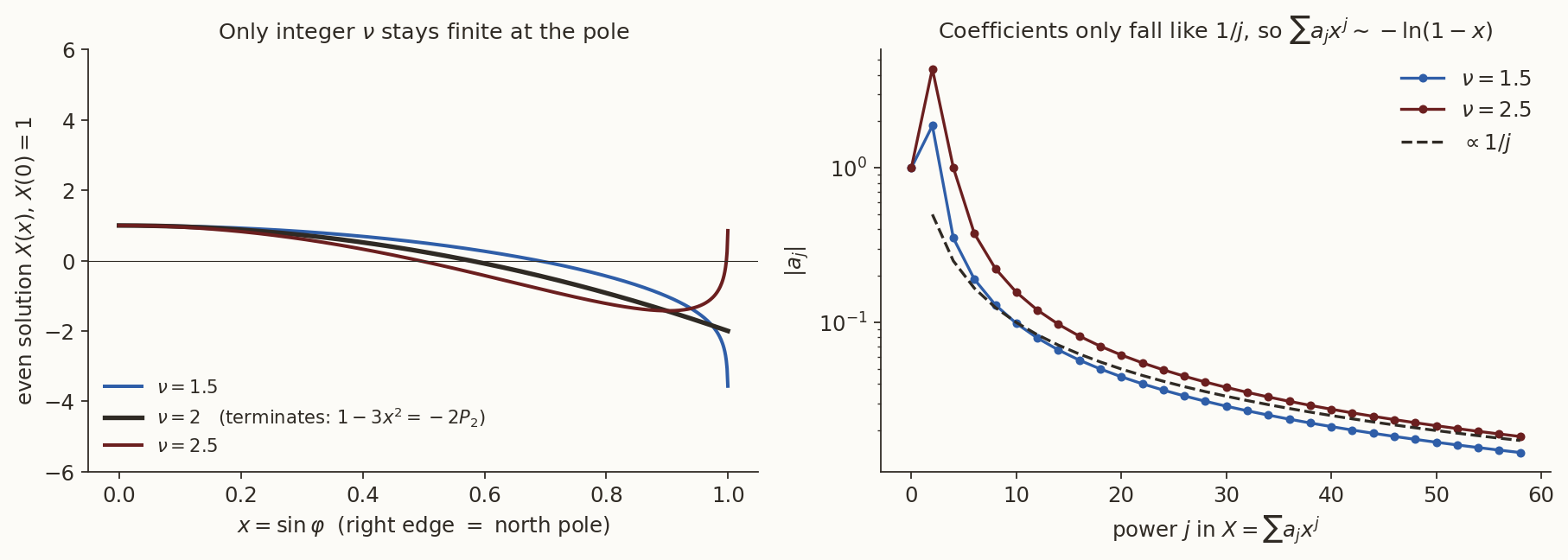
So regularity at the poles quantises the separation constant: \(k=n(n+1)\) with \(n=0,1,2,\dots\), and the latitude functions are the Legendre polynomials \(P_n\). This is why the same polynomials appear in the two routes: the terms of Equation 5 are of the form \(r^{-(n+1)}P_n(\cos\gamma)\) with the polar axis along \(\mathbf r'\), and they must solve Laplace’s equation term by term (they are the separable solutions).

(d) Latitude with \(m>0\). For \(m\neq0\) the equation is \[ \bigl[(1-x^2)X'\bigr]'+\Bigl[n(n+1)-\frac{m^2}{1-x^2}\Bigr]X=0 . \tag{22}\] Its regular solutions are the associated functions of Equation 8, \(X=P_{nm}(x)=(1-x^2)^{m/2}\,d^mP_n/dx^m\). Verification for the simplest case \(n=m=1\): \(X=\sqrt{1-x^2}\), \(X'=-x(1-x^2)^{-1/2}\), \((1-x^2)X'=-x(1-x^2)^{1/2}\), and \[ \bigl[(1-x^2)X'\bigr]'=-(1-x^2)^{1/2}+x^2(1-x^2)^{-1/2}, \] \[ \Bigl[2-\tfrac{1}{1-x^2}\Bigr]X=2(1-x^2)^{1/2}-(1-x^2)^{-1/2}. \] The sum is \((1-x^2)^{1/2}-(1-x^2)^{-1/2}(1-x^2)=0\). ✓ Solutions exist and are finite at the poles only if \(m\le n\); for \(m>n\) the \(m\)th derivative of a degree-\(n\) polynomial is zero.

6.5 Putting it together: the complete list

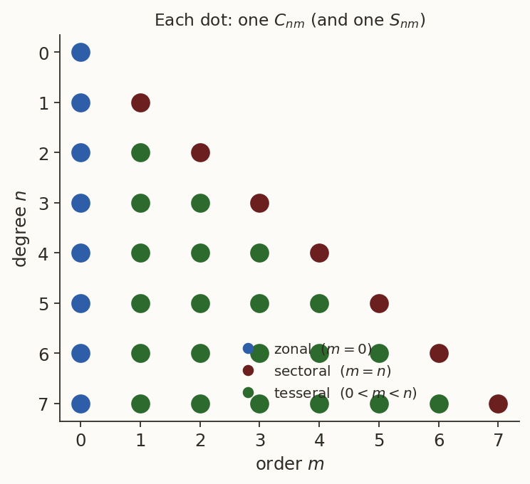
For each degree \(n\), the separable solutions that decay at infinity and are regular everywhere on the sphere are \[ \frac{1}{r^{n+1}}\,P_{nm}(\sin\varphi)\begin{Bmatrix}\cos m\lambda\\ \sin m\lambda\end{Bmatrix},\qquad m=0,1,\dots,n\quad(\text{only }\cos\text{ for }m=0), \] that is \(2n+1\) independent functions for each \(n\) (Figure 9). A general exterior potential is a linear combination of all of them, which is Equation 10. Nothing else can appear. What Laplace’s equation cannot tell us is the weights; that is what the mass integrals of Equation 11 (and satellite tracking) supply.

Figure 9: The set of coefficients. Each dot is a pair \((C_{nm},S_{nm})\); the dots with \(m=0\) are the zonal \(J_n\) (bands of latitude), those with \(m=n\) are sectoral, and the rest tesseral. Degree \(n\) has \(2n+1\) free numbers. Script: fig-grav-harmonics.py.

Orthogonality. The Legendre polynomials satisfy \(\int_{-1}^{1}P_nP_{n'}\,dx=\frac{2}{2n+1}\delta_{nn'}\) (e.g. \(\int_{-1}^1x\cdot\tfrac12(3x^2-1)dx=0\)). Together with the \(\cos m\lambda,\sin m\lambda\) orthogonality, this means each coefficient can be isolated by projecting the measured potential onto its function. That is how gravity fields such as EGM96 and EGM2008 are extracted from tracking data: as a big linear least-squares problem for the \(C_{nm},S_{nm}\).

6.6 What the functions look like

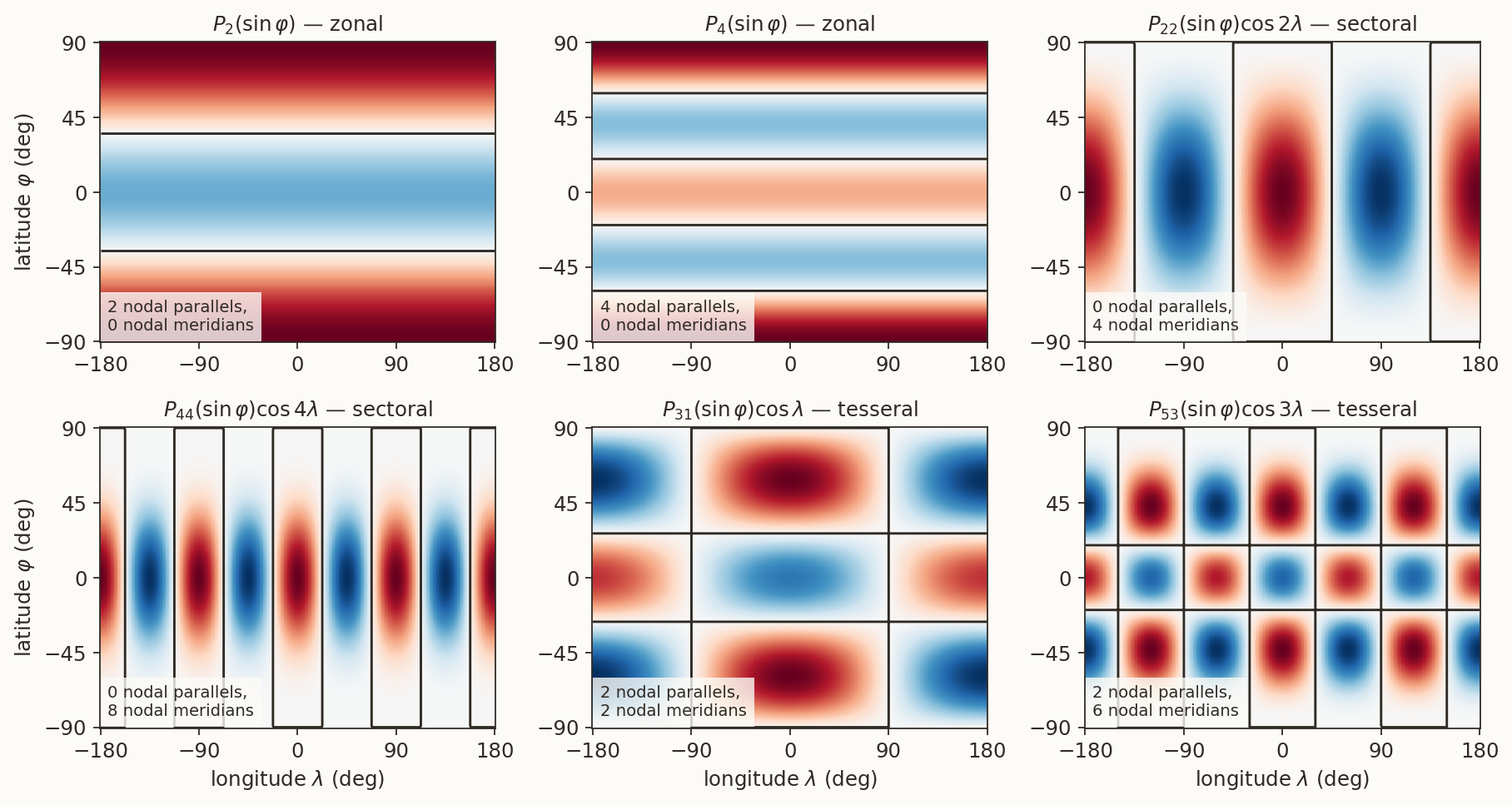
Figure 10 shows \(P_{nm}(\sin\varphi)\cos m\lambda\) on a latitude–longitude map, so you can see what each “term” does to the potential. The number of sign changes is \(n-m\) along a meridian and \(2m\) along a parallel.

• Zonal (\(m=0\)): bands of latitude. \(J_2\) is the pattern “positive at the poles, negative in the equatorial belt”; the extra minus sign in Equation 13 turns this into “more potential at the equator”.
• Sectoral (\(m=n\)): slices of longitude like orange segments; \(C_{22},S_{22}\) are the \(n=m=2\) case (four sectors: the equator is slightly elliptical).
• Tesseral (\(0<m<n\)): chequerboards.

Figure 10: Real spherical-harmonic patterns \(P_{nm}(\sin\varphi)\cos m\lambda\) normalised to unit peak amplitude. Red positive, blue negative, black lines mark sign changes. Top row: two zonal harmonics and the \(n=m=2\) sectoral harmonic. Bottom row: a higher sectoral and two tesseral harmonics. Script: fig-grav-harmonics.py.

7 The Earth’s actual coefficients

Modern models (EGM96, EGM2008) list thousands of coefficients: EGM2008 is complete to degree and order \(2159\). For orbit dynamics we need very few.

Table 3: Selected (unnormalised) coefficients.

Coefficient	Value	Meaning
\(J_2\)	\(+1.08263\times10^{-3}\)	oblateness (Equation 14)
\(J_3\)	\(-2.5327\times10^{-6}\)	north–south asymmetry (“pear shape”)
\(J_4\)	\(-1.6196\times10^{-6}\)	flattening’s second-order shape
\(C_{22},\,S_{22}\)	\(1.5745\times10^{-6},\ -9.0387\times10^{-7}\)	equatorial ellipticity (Equation 15)

History. On 17 March 1958 the US launched Vanguard 1. Analysis of the small, periodic variation in its eccentricity (O’Keefe and colleagues, 1959) revealed a non-zero \(J_3\): the Earth is slightly pear-shaped, with a fatter southern hemisphere. The nodal regression of Sputnik and early Explorer satellites had already shown that \(J_2\) was larger than pre-space geodesy suggested.

Figure 11: How big are the terms? Relative to the point-mass term (\(=1\)), \(J_2\) is a thousandth, while every other coefficient is a few millionths, roughly following Kaula’s rule of thumb (dashed; strictly for normalised coefficients) that the size of degree-\(n\) terms falls like \(10^{-5}/n^{2}\). Script: fig-grav-earth.py.

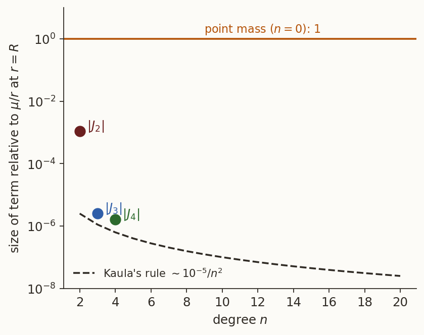
Figure 11 shows the crucial point: \(J_2\) is about \(400\) times larger than the general trend (the next largest terms, \(J_3,J_4,C_{22},\dots\), are of order \(10^{-6}\)). That is why nearly all of orbit theory first keeps just the point mass and \(J_2\).

Why so large? A rotating fluid body must flatten: gravity plus the centrifugal potential \(\tfrac12\omega^2\rho^2\) have to be balanced by the shape. To first order in the small quantities, Clairaut’s theory gives \[ J_2\approx\frac{2f-m}{3},\qquad f=\tfrac1{298.257},\quad m=\frac{\omega^2R^3}{\mu}=3.461\times10^{-3}, \] which yields \(1.081\times10^{-3}\), remarkably close to the measured value. So \(J_2\) is big because of the Earth’s spin, while the other coefficients come from geology (mountains, mantle convection, ocean basins) and are typically \(10^{-6}\).

8 The \(J_2\) potential and acceleration

From now on keep only the point mass and \(J_2\). With \(P_2(\sin\varphi)=\tfrac12(3\sin^2\varphi-1)\), Equation 13 gives \[ U=\frac{\mu}{r}+\mathcal R,\qquad \boxed{\ \mathcal R=-\frac{\mu J_2R^{2}}{2r^{3}}\bigl(3\sin^2\varphi-1\bigr)\ } \tag{23}\] where \(\mathcal R\) is the perturbing potential (disturbing function). Since \(\mathbf a=\nabla U\), \[ \ddot{\mathbf r}=-\frac{\mu}{r^3}\mathbf r+\nabla\mathcal R . \]

8.1 Turning the potential into Cartesian components

Perform all differentiations in the Earth-centred inertial frame, with \(z\) along the spin axis. The latitude satisfies \(\sin\varphi=z/r\), so \[ \mathcal R=-\frac{\mu J_2R^2}{2}\Bigl(\frac{3z^2}{r^5}-\frac1{r^3}\Bigr). \] We differentiate using \(\partial r/\partial x=x/r\), \(\partial r/\partial z=z/r\):

• \(\dfrac{\partial}{\partial x}\Bigl(\dfrac{3z^2}{r^5}-\dfrac1{r^3}\Bigr)=-\dfrac{15xz^2}{r^7}+\dfrac{3x}{r^5}=\dfrac{3x}{r^5}\Bigl(1-\dfrac{5z^2}{r^2}\Bigr)\),
• \(\dfrac{\partial}{\partial z}\Bigl(\dfrac{3z^2}{r^5}-\dfrac1{r^3}\Bigr)=\dfrac{6z}{r^5}-\dfrac{15z^3}{r^7}+\dfrac{3z}{r^5}=\dfrac{3z}{r^5}\Bigl(3-\dfrac{5z^2}{r^2}\Bigr)\).

The \(y\) derivative is the same as \(x\) with \(x\to y\). Multiplying by \(-\mu J_2R^2/2\): \[ \boxed{\begin{aligned} a_x&=-\frac{3}{2}\,\frac{\mu J_2R^{2}}{r^{5}}\;x\Bigl(1-\frac{5z^{2}}{r^{2}}\Bigr)\\ a_y&=-\frac{3}{2}\,\frac{\mu J_2R^{2}}{r^{5}}\;y\Bigl(1-\frac{5z^{2}}{r^{2}}\Bigr)\\ a_z&=-\frac{3}{2}\,\frac{\mu J_2R^{2}}{r^{5}}\;z\Bigl(3-\frac{5z^{2}}{r^{2}}\Bigr) \end{aligned}} \tag{24}\] This is the acceleration you would code into a propagator. Note the asymmetry between \(z\) and \((x,y)\): it is not a central force, and it does not point along \(\mathbf r\).

8.2 Spherical components, and what they mean

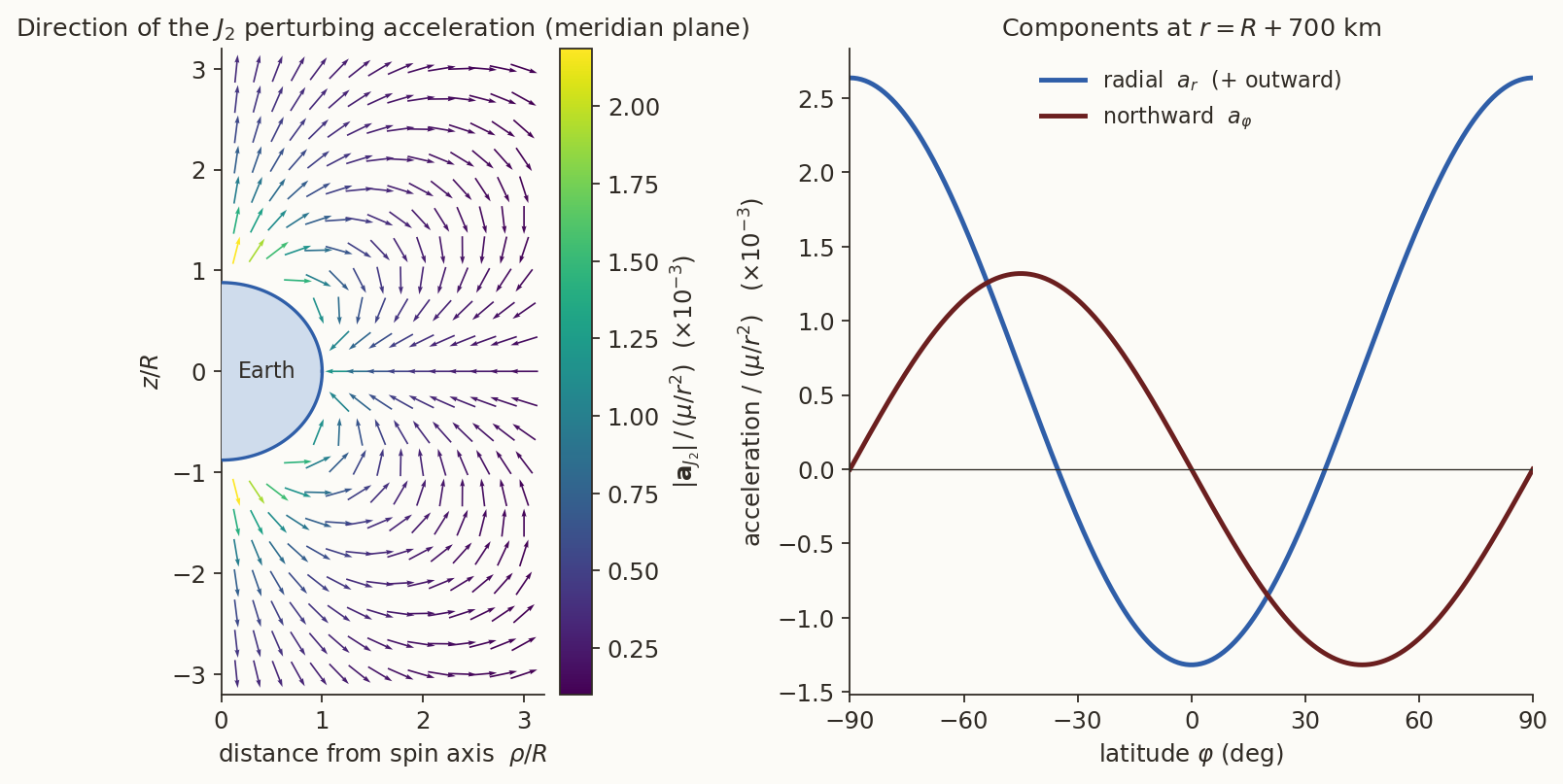
Alternatively differentiate Equation 23 in spherical coordinates. The gradient components are \(\partial_r\), \(\frac1r\partial_\varphi\): \[ \boxed{\ a_r=\frac{\partial\mathcal R}{\partial r}=\frac{3\mu J_2R^2}{2r^4}\bigl(3\sin^2\varphi-1\bigr),\qquad a_\varphi=\frac1r\frac{\partial\mathcal R}{\partial\varphi}=-\frac{3\mu J_2R^2}{2r^4}\sin2\varphi\ } \tag{25}\] (using \(\frac{d}{d\varphi}(3\sin^2\varphi-1)=6\sin\varphi\cos\varphi=3\sin2\varphi\)). One can check numerically that \(a_x\hat{\mathbf x}+a_y\hat{\mathbf y}+a_z\hat{\mathbf z}=a_r\hat{\mathbf r}+a_\varphi\hat{\boldsymbol\varphi}\) (we did, to machine precision, when drawing Figure 12). The spherical form has a simple physical reading:

• At the equator (\(\varphi=0\)): \(a_r=-\frac{3\mu J_2R^2}{2r^4}<0\): an extra inward pull, as expected from nearby extra mass in the equatorial belt.
• Over the poles (\(\varphi=\pm90^\circ\)): \(a_r=+\frac{3\mu J_2R^2}{r^4}>0\): gravity is weaker than the point mass, because mass was moved from there to the equator.
• \(a_\varphi\) has the sign of \(-\varphi\) times something positive: it points toward the equator in both hemispheres and is largest at \(45^\circ\). This is the sideways tug drawn in Figure 1.

The size relative to the point-mass acceleration \(\mu/r^2\) is \(\frac32J_2(R/r)^2\times O(1)\). At \(r=R+700\) km that is \(1.3\times10^{-3}\) at the equator: \(a\approx0.010\ \text{m/s}^2\) against \(7.96\ \text{m/s}^2\). It looks negligible, but acting for one orbit (\(\sim5900\) s) it could displace a satellite by \(\tfrac12at^2\sim10^2\) km, far more than any tolerance in tracking, and it acts always in the same sense.

Figure 12: The \(J_2\) perturbing acceleration. Left: directions in a meridian plane (arrow colour = magnitude relative to \(\mu/r^2\)). Near the equator the vectors point inward; over the poles outward; in between they tilt toward the equatorial plane. Right: the radial and northward components at \(r=R+700\) km, straight from Equation 25. Script: fig-grav-earth.py.

9 What \(J_2\) does to an orbit

9.1 A physical picture: torque on the orbit plane

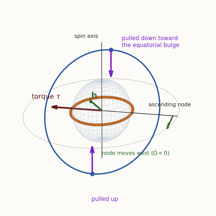
Think of the orbit as a ring of mass. The equatorial bulge pulls the part of the ring that is above the equatorial plane down, and the part below it up, as in Figure 13. The forces are the ones in Figure 12. These forces exert a torque on the orbit. A torque tends to tilt the angular momentum \(\mathbf h\); but \(\mathbf h\) is spinning, so like a gyroscope (or a spinning top under gravity) it does not fall over: it precesses. The precession axis is the Earth’s spin axis, so the orbital plane turns about the polar axis, and the node \(\Omega\) drifts.

Figure 13: Why the plane precesses. The equatorial bulge pulls the upper arc of the orbit down and the lower arc up. Both forces produce a torque along the line of nodes (here \(-\hat{\mathbf x}\)), which is perpendicular to both \(\mathbf h\) and the spin axis. A torque perpendicular to \(\mathbf h\) turns \(\mathbf h\) without changing its length: the plane rotates westward (for prograde orbits). Script: fig-grav-orbit.py.

We now make this exact. The rate of change of the specific angular momentum \(\mathbf h=\mathbf r\times\mathbf v\) is \[ \dot{\mathbf h}=\mathbf r\times\ddot{\mathbf r}=\underbrace{\mathbf r\times\Bigl(-\frac{\mu}{r^3}\mathbf r\Bigr)}_{=0}+\mathbf r\times\nabla\mathcal R\equiv\boldsymbol\tau . \tag{26}\] (The point-mass term is parallel to \(\mathbf r\) and gives no torque; this is angular-momentum conservation.)

Evaluating \(\boldsymbol\tau\). In Equation 23, \(\mathcal R\) depends on position through two variables, \(r\) and \(z\). By the chain rule, with \(\nabla r=\hat{\mathbf r}\) and \(\nabla z=\hat{\mathbf z}\), \[ \nabla\mathcal R=\frac{\partial\mathcal R}{\partial r}\Big|_z\hat{\mathbf r}+\frac{\partial\mathcal R}{\partial z}\Big|_r\hat{\mathbf z}. \] The first part is parallel to \(\mathbf r\) and gives no torque. For the second, \(\frac{\partial\mathcal R}{\partial z}\big|_r=-\frac{\mu J_2R^2}{2}\frac{6z}{r^5}=-\frac{3\mu J_2R^2z}{r^5}\), and \(\mathbf r\times\hat{\mathbf z}=(y,-x,0)\). Hence \[ \boldsymbol\tau=-\frac{3\mu J_2R^2\,z}{r^{5}}\,(y,\,-x,\,0). \tag{27}\] Two things follow instantly. First, \(\tau_z=0\) exactly, so \(h_z=h\cos i\) is constant: the potential is symmetric about the spin axis. Second, \(\boldsymbol\tau\perp\hat{\mathbf z}\), and it is also perpendicular to \(\mathbf r\): the torque lies in the equatorial plane.

Orbit average. The torque oscillates within each orbit; the lasting effect is its average over one period. Choose axes so that, at the instant considered, the line of nodes is along \(x\) (so \(\Omega=0\)). With \(u=\omega+\nu\) the argument of latitude, \[ x=r\cos u,\qquad y=r\sin u\cos i,\qquad z=r\sin u\sin i . \] Substituting in Equation 27: \[ \tau_x=-\frac{3\mu J_2R^2}{r^{3}}\sin i\cos i\,\sin^2u,\qquad \tau_y=\frac{3\mu J_2R^2}{r^{3}}\sin i\,\sin u\cos u . \]

Time averages. Angular momentum gives \(r^2\dot\nu=h=na^2\sqrt{1-e^2}\), so \(dt=\dfrac{r^2\,d\nu}{na^2\sqrt{1-e^2}}\) and, with \(p=a(1-e^2)\) and \(r=p/(1+e\cos\nu)\), \[ \Bigl\langle\frac{f}{r^3}\Bigr\rangle\equiv\frac1T\!\int_0^Tf\,\frac{dt}{r^3}=\frac{1}{2\pi a^2\sqrt{1-e^2}}\int_0^{2\pi}f\,\frac{d\nu}{r}=\frac{1}{2\pi a^2\sqrt{1-e^2}\,p}\int_0^{2\pi}f\,(1+e\cos\nu)\,d\nu . \] * With \(f=1\): \(\langle r^{-3}\rangle=\dfrac{2\pi}{2\pi a^2\sqrt{1-e^2}\,p}=\dfrac{1}{a^{3}(1-e^2)^{3/2}}\). * With \(f=\sin^2u=\tfrac12[1-\cos(2\nu+2\omega)]\): \(\int_0^{2\pi}\cos(2\nu+2\omega)(1+e\cos\nu)\,d\nu=0\) (the product \(\cos\nu\cos(2\nu+2\omega)=\tfrac12[\cos(3\nu+2\omega)+\cos(\nu+2\omega)]\) also integrates to zero), so \(\langle\sin^2u/r^3\rangle=\tfrac12\langle r^{-3}\rangle\). * With \(f=\sin u\cos u=\tfrac12\sin(2\nu+2\omega)\): the integral vanishes by the same argument, \(\langle\sin u\cos u/r^3\rangle=0\).

(For a circular orbit these are trivial: \(r\) is constant and \(\langle\sin^2u\rangle=\tfrac12\), \(\langle\sin u\cos u\rangle=0\).) Therefore \[ \langle\tau_x\rangle=-\frac{3\mu J_2R^2\sin i\cos i}{2\,a^3(1-e^2)^{3/2}},\qquad\langle\tau_y\rangle=0,\qquad\langle\tau_z\rangle=0 . \]

From torque to rates. In the same instant, the angular-momentum vector is \(\mathbf h=h(\sin i\sin\Omega,\ -\sin i\cos\Omega,\ \cos i)\). Differentiate and set \(\Omega=0\): \[ \dot h_x=h\sin i\,\dot\Omega,\qquad\dot h_y=-\frac{d(h\sin i)}{dt},\qquad\dot h_z=\frac{d(h\cos i)}{dt}. \] Equating averages with \(\langle\boldsymbol\tau\rangle\): \(\langle\dot h_y\rangle=0\) and \(\langle\dot h_z\rangle=0\) mean that both \(h\sin i\) and \(h\cos i\) are constant, so \(h\) and \(i\) have no secular drift. And \[ h\sin i\,\dot\Omega=\langle\tau_x\rangle\quad\Rightarrow\quad \dot\Omega=-\frac{3\mu J_2R^2\cos i}{2\,h\,a^{3}(1-e^2)^{3/2}} . \] Use \(h=na^2\sqrt{1-e^2}\) and \(\mu=n^2a^3\): \[ \boxed{\ \dot\Omega=-\frac{3}{2}\,\frac{J_2R^{2}}{a^{2}(1-e^{2})^{2}}\;n\cos i\ } \tag{28}\] The node regresses (moves westward) for prograde orbits (\(i<90^\circ\)), advances for retrograde, and does not move for polar orbits (\(\cos i=0\)). This matches the picture in Figure 13.

9.2 The rotation of the perigee

The perigee direction obeys a similar but more laborious equation (it involves the eccentricity vector, not just \(\mathbf h\)). We use the Lagrange planetary equations, which give the rates of the orbital elements directly from the perturbing potential \(\mathcal R\) (derived in the chapter on general perturbations): \[ \dot\Omega=\frac{1}{na^2\sqrt{1-e^2}\,\sin i}\frac{\partial\mathcal R}{\partial i},\qquad \dot\omega=\frac{\sqrt{1-e^2}}{na^2e}\frac{\partial\mathcal R}{\partial e}-\frac{\cos i}{na^2\sqrt{1-e^2}\,\sin i}\frac{\partial\mathcal R}{\partial i}. \] As before, keep only the orbit average. Using \(\sin\varphi=\sin i\sin u\) in Equation 23 and the averages just computed, \[ \langle\mathcal R\rangle=-\frac{\mu J_2R^2}{2}\Bigl[3\sin^2i\,\Bigl\langle\frac{\sin^2u}{r^3}\Bigr\rangle-\Bigl\langle\frac1{r^3}\Bigr\rangle\Bigr] =\frac{\mu J_2R^2}{4a^3(1-e^2)^{3/2}}\bigl(3\cos^2i-1\bigr), \] where \(3\sin^2 i/2-1=-(3\cos^2 i-1)/2\) was used. With \(\mu=n^2a^3\) the derivatives are \[ \frac{\partial\langle\mathcal R\rangle}{\partial i}=-\frac{6\,n^2J_2R^2\sin i\cos i}{4(1-e^2)^{3/2}},\qquad \frac{\partial\langle\mathcal R\rangle}{\partial e}=\frac{3e\,n^2J_2R^2\,(3\cos^2i-1)}{4(1-e^2)^{5/2}} . \] Check on \(\dot\Omega\): the first Lagrange equation gives \(\dot\Omega=\frac{1}{na^2\sqrt{1-e^2}\sin i}\cdot\bigl(-\frac{6n^2J_2R^2\sin i\cos i}{4(1-e^2)^{3/2}}\bigr)=-\frac32\frac{nJ_2R^2\cos i}{a^2(1-e^2)^2}\). ✓ It agrees with the torque calculation, Equation 28. For the perigee: \[ \dot\omega=\underbrace{\frac{3nJ_2R^2(3\cos^2i-1)}{4a^2(1-e^2)^{2}}}_{\text{from }\partial_e}+\underbrace{\frac{6nJ_2R^2\cos^2i}{4a^2(1-e^2)^2}}_{\text{from }\partial_i} =\frac{nJ_2R^2}{4a^2(1-e^2)^2}\bigl(15\cos^2i-3\bigr), \] \[ \boxed{\ \dot\omega=\frac{3}{4}\,\frac{J_2R^{2}}{a^{2}(1-e^{2})^{2}}\;n\,\bigl(5\cos^2i-1\bigr)\ } \tag{29}\] This vanishes when \(5\cos^2i=1\), i.e. \(\cos i=\pm1/\sqrt5\), at the critical inclinations \(i=63.435^\circ\) and \(116.565^\circ\).

History. The critical inclination was recognised in the late 1950s in the analyses by Brouwer and Kozai of Earth-satellite theory. It became an engineering tool when the Soviet Molniya orbits (\(i\approx63.4^\circ\), \(e\approx0.74\), 12-hour period, first launched 1965) were designed so that the apogee stays over the northern hemisphere for years without fuel-costly correction.

9.3 Consequences

Figure 14 collects the results.

Figure 14: Left: nodal drift rate against inclination for circular orbits at several altitudes (it vanishes for polar orbits; at GEO it is nearly zero). The dashed line is the rate needed to follow the mean Sun. Middle: the inclination for which \(\dot\Omega\) equals that Sun-following rate. Right: the perigee drift changes sign at \(63.4^\circ\) and \(116.6^\circ\). Script: fig-grav-orbit.py.

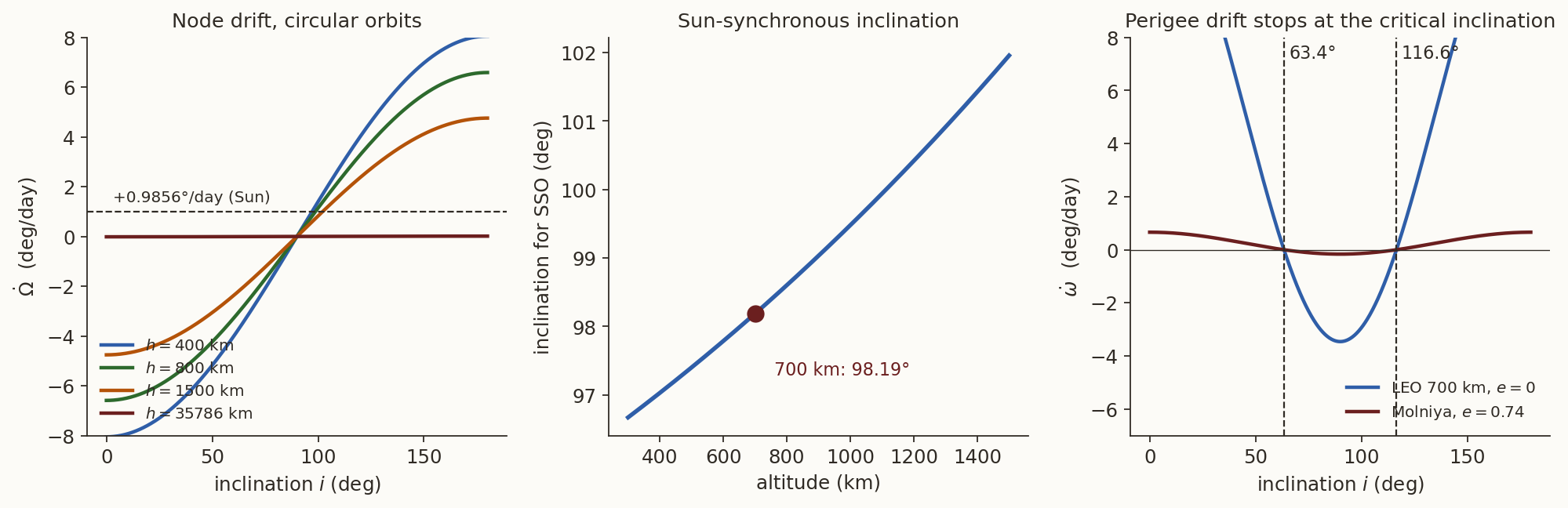
• ISS (\(h\approx420\) km, \(i=51.6^\circ\)): Equation 28 gives \(\dot\Omega\approx-4.95^\circ\)/day, so the plane turns once in about 73 days.
• Sun-synchronous orbits. The Sun’s mean apparent motion is \(360^\circ/365.2422\,\text{d}=+0.9856^\circ\)/day. Setting \(\dot\Omega\) equal to this fixes \(\cos i=-\dfrac{2a^2(1-e^2)^2\dot\Omega_\odot}{3nJ_2R^2}\), which is negative: the orbit must be slightly retrograde. At \(h=700\) km, \(i=98.19^\circ\). Earth-observation satellites use this so that the local solar time at which they cross a given latitude stays fixed and shadows are consistent from pass to pass.
• Critical inclination (\(63.4^\circ\)): \(\dot\omega=0\). Molniya and Tundra orbits use it to keep apogee over Russia/Canada.
• GPS (20 200 km, \(55^\circ\)): \(\dot\Omega\approx-0.039^\circ\)/day; small, but not negligible over years.

9.4 A numerical experiment

Are we sure of all of this? Integrate the full equations of motion \(\ddot{\mathbf r}=-\mu\mathbf r/r^3+\nabla\mathcal R\) (with Equation 24) for five days for \(a=8000\) km, \(e=0.1\), \(i=50^\circ\), \(\Omega_0=40^\circ\), \(\omega_0=30^\circ\); at each step convert \((\mathbf r,\mathbf v)\) to the osculating elements and compare with Equation 28 and Equation 29.

Figure 15: Numerical integration of the \(J_2\) problem (blue) against the linear secular formulae (dashed). The osculating elements ripple around the secular trend with the orbital period, but the trend is captured. The inclination has no secular drift. Script: fig-grav-orbit.py.

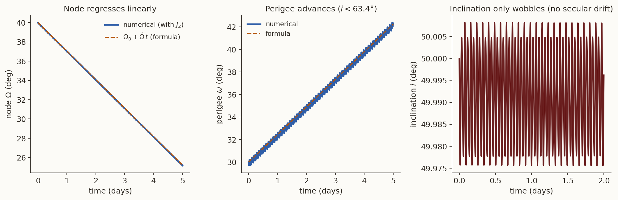
The fitted slopes are \(\dot\Omega=-2.964^\circ\)/day (formula: \(-2.957\)) and \(\dot\omega=+2.459^\circ\)/day (formula: \(+2.452\)): agreement to \(\approx0.2\%\). The remainder comes from the short-period terms, from the difference between osculating and mean \(a\) (which enters \(n\) and the prefactor), and from terms of order \(J_2^2\) that the first-order averaging neglects.

10 Beyond \(J_2\): the tesseral harmonics and geostationary drift

Longitude-dependent terms make the field different at different longitudes. For an inertial-frame orbit these terms average out because the Earth rotates beneath the satellite, unless the satellite rotates with the Earth, as in a geostationary orbit. Then the satellite feels the same longitude-dependent force all the time.

The relevant term is \(n=m=2\). At the equator (\(\varphi=0\)) \(P_{22}(0)=3\), so from Equation 10 \[ U_{22}=\frac{3\mu R^2}{r^3}\bigl(C_{22}\cos2\lambda+S_{22}\sin2\lambda\bigr)=\frac{3\mu R^2J_{22}}{r^3}\cos2(\lambda-\lambda_{22}), \] where we combined the two terms: \(J_{22}=\sqrt{C_{22}^2+S_{22}^2}=1.816\times10^{-6}\) and \(2\lambda_{22}=\operatorname{atan2}(S_{22},C_{22})\), i.e. \(\lambda_{22}=-14.9^\circ\) (the longitude of the Earth’s long equatorial axis, \(14.9^\circ\)W; the cosine identity is \(\cos2\lambda\cos2\lambda_{22}+\sin2\lambda\sin2\lambda_{22}=\cos2(\lambda-\lambda_{22})\)).

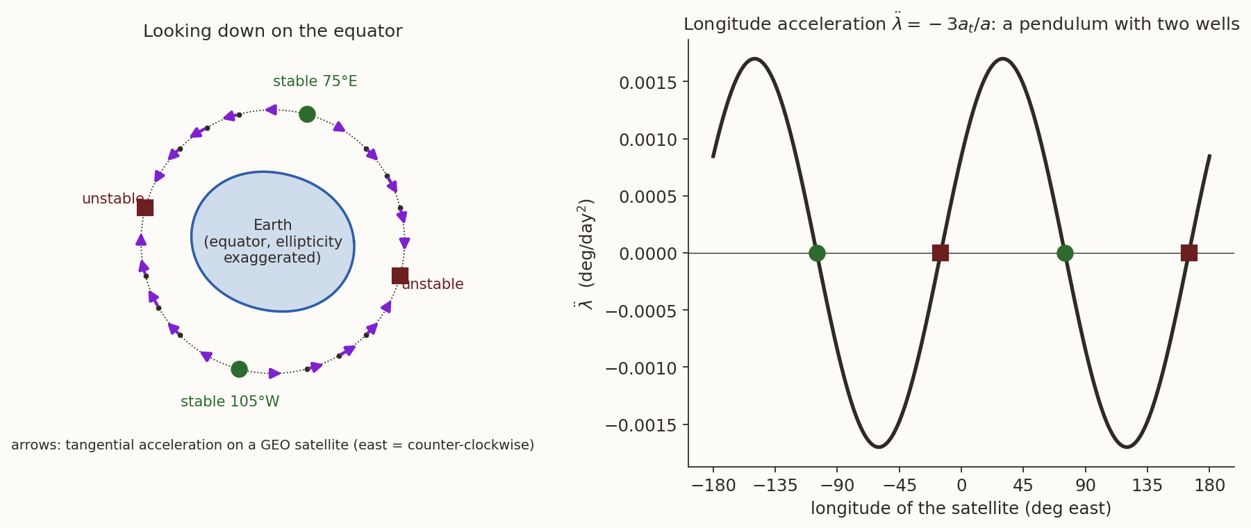
Tangential acceleration. The eastward acceleration component is \(\frac{1}{r\cos\varphi}\partial_\lambda U\) (the \(\lambda\)-component of \(\nabla U\); \(h_\lambda=r\cos\varphi\)): \[ a_t=\frac1r\frac{\partial U_{22}}{\partial\lambda}=-\frac{6\mu R^2J_{22}}{r^{4}}\,\sin2(\lambda-\lambda_{22}). \] This acceleration points toward the nearest bulge (arrows in Figure 16, left).

Turning \(a_t\) into drift. For a nearly circular orbit, the specific energy is \(E=-\mu/2a\) and \(\dot E=\mathbf v\cdot\mathbf a=v\,a_t\), so \(\dot a=\frac{2a^2}{\mu}v\,a_t=\frac{2a_t}{n}\) (using \(v=na\)). The satellite’s angular rate is \(n=\sqrt{\mu/a^3}\), so \(\dot n=-\tfrac32\frac na\dot a=-\frac{3a_t}{a}\). The longitude of a satellite in the rotating Earth frame changes at \(\dot\lambda=n-\omega_\oplus\), hence \[ \ddot\lambda=-\frac{3a_t}{a}=\frac{18\mu R^2J_{22}}{a^{5}}\,\sin2(\lambda-\lambda_{22}) . \tag{30}\] Counter-intuitively, the sign is reversed: a push forward raises the orbit, which slows the satellite’s angular rate, so it falls behind. The satellite is repelled from the direction of the bulge in longitude.

Equilibria. \(\ddot\lambda=0\) when \(\sin2(\lambda-\lambda_{22})=0\), i.e. at \(\lambda=\lambda_{22}+k\cdot90^\circ\). An equilibrium is stable if \(\ddot\lambda\) decreases with increasing \(\lambda\) across it, i.e. \(\cos2(\lambda-\lambda_{22})<0\), which selects \(\lambda_{22}\pm90^\circ\):

• Stable: \(75.1^\circ\)E and \(104.9^\circ\)W. (A satellite parked there needs little east–west station-keeping.)
• Unstable: \(14.9^\circ\)W and \(165.1^\circ\)E.

For \(a=42\,164\) km the peak \(|\ddot\lambda|=18\mu R^2J_{22}/a^5=3.98\times10^{-15}\) rad/s\(^2=1.70\times10^{-3}\) deg/day\(^2\). Small oscillations about a stable point have \(\omega_{\rm lib}^2=2\times3.98\times10^{-15}\ \text{s}^{-2}\), i.e. a libration period of about \(2.2\) years. A satellite parked away from a stable point drifts and needs east–west station-keeping burns; near it, the satellite just rocks slowly.

Figure 16: Left: looking down on the equator, with the ellipticity exaggerated. Purple arrows show the tangential acceleration on a GEO satellite, always pointing toward the nearest bulge. Right: \(\ddot\lambda\) versus longitude from Equation 30: a “double pendulum”, with stable points (green) at \(75^\circ\)E and \(105^\circ\)W and unstable points (red squares) at the ends of the long axis. Script: fig-grav-earth.py.

11 Summary

The chain of reasoning

1. Use the scalar potential \(U=G\int dm'/s\): superposition is a plain sum. (Section 3)
2. Expand \(1/s\) in \(\varepsilon=r'/r<1\): the coefficients are Legendre polynomials (Equation 3); this separates the field point from the mass element. (Section 4)
3. Express \(\cos\gamma\) through latitude and longitude with the addition theorem; this gives \(P_{nm}(\sin\varphi)\cos m\lambda\), \(\sin m\lambda\) times numbers \(C_{nm},S_{nm}\) that are moments of the mass distribution (Equation 11), e.g. \(J_2=[C-\tfrac12(A+B)]/MR^2\). (Section 5)
4. Laplace’s equation + separation of variables shows the same functions are the complete set: \(m\) integer (periodicity), \(r^{-(n+1)}\) (decay), \(n\) integer (finiteness at the poles). (Section 6)
5. Keep \(J_2\): \(\mathcal R=-\frac{\mu J_2R^2}{2r^3}(3\sin^2\varphi-1)\), giving the acceleration Equation 24. (Section 8)
6. Orbit-average the torque: \(\dot\Omega=-\frac32nJ_2(R/p)^2\cos i\) and \(\dot\omega=\frac34nJ_2(R/p)^2(5\cos^2i-1)\) with \(p=a(1-e^2)\); no secular change in \(a,e,i\). (Section 9)
7. \(C_{22},S_{22}\) give the longitude-dependent force that makes GEO satellites drift toward \(75^\circ\)E and \(105^\circ\)W. (Section 10)

What we left out. (i) Higher zonals and tesserals (\(J_3,J_4,\dots\)) produce small long-period effects, notably a slow oscillation of \(e\) and \(\omega\) (\(J_3\)), and are included in numerical propagators as truncated sums of Equation 10, evaluated with recurrence relations like Equation 4. (ii) Second-order \(J_2\) effects and short-period terms (Kozai 1959, Brouwer 1959) improve the accuracy of \(\dot\Omega,\dot\omega\) and of the mean motion. (iii) Non-gravitational and third-body effects: atmospheric drag, solar radiation pressure, and the Sun and Moon, matter as much as \(J_2\) at high altitude. (iv) Time-variable gravity (ice sheets, groundwater) is measured by missions such as GRACE (2002–2017) and its successors.

Further reading. R. H. Battin, An Introduction to the Mathematics and Methods of Astrodynamics (the sections on the Earth’s gravitational potential and on perturbation theory); D. Vallado, Fundamentals of Astrodynamics and Applications (the chapter on perturbations); W. M. Kaula, Theory of Satellite Geodesy (1966); B. Hofmann-Wellenhof and H. Moritz, Physical Geodesy.

12 Exercises

1. Legendre by recurrence. Use Equation 4 to obtain \(P_5(x)\) and verify that \(P_5(1)=1\). Check that \(P_3\) satisfies Legendre’s equation Equation 20 with \(n=3\).
2. Ring on the axis, second look. Repeat the ring calculation for a field point in the equatorial plane at distance \(r>a\). Which \(\gamma\) applies now, and what is the sign of the \(n=2\) term compared with the axis case? Explain it physically.
3. MacCullagh at the pole and the equator. For an axisymmetric body (\(A=B\)) evaluate Equation 6 at a point on the polar axis (the line \(OP\) is the \(z\)-axis, so \(I=C\)) and at a point in the equatorial plane (the line \(OP\) is an equatorial axis, so \(I=A\)). Show that \(U_2=\dfrac{G(A-C)}{r^3}\) on the axis and \(U_2=\dfrac{G(C-A)}{2r^3}\) in the equatorial plane. Compare with \(-\frac{\mu}{r}J_2(R/r)^2P_2(\sin\varphi)\).
4. Acceleration at a point. A satellite is at \(\mathbf r=(4500,\,3000,\,5000)\) km. Compute \(a_x,a_y,a_z\) from Equation 24 and its radial and northward components from Equation 25. Confirm that both give the same vector.
5. Polar orbits. Show from Equation 28 that a polar orbit has \(\dot\Omega=0\), and from Equation 29 that its perigee rotates at \(-\tfrac34nJ_2(R/p)^2\). Why is a Sun-synchronous orbit necessarily retrograde?
6. Design. Find the altitude of a circular Sun-synchronous orbit with \(i=98.6^\circ\) (use Equation 28; a root-finding step is needed). Answer: about \(800\) km.
7. GEO libration. A satellite is at \(\lambda=60^\circ\)E. Compute \(\ddot\lambda\) from Equation 30 and predict the drift after \(30\) days if it starts with \(\dot\lambda=0\). Which direction does it drift?
8. Uniform Earth. Using the homogeneous spheroid result \(J_2=(a^2-c^2)/(5a^2)\), what would the inertia ratio \(C/(MR^2)\) have to be to reproduce the observed \(J_2\) with \((C-A)/C=1/305.4\)? Compare with the uniform value \(0.4\) and comment.

13 Appendix: Legendre polynomials as Taylor coefficients

Fix a number \(x\in[-1,1]\) and define \(f_x(\varepsilon)=(1-2x\varepsilon+\varepsilon^2)^{-1/2}\). For this fixed \(x\), \(f_x\) is an ordinary function of the single variable \(\varepsilon\), analytic near \(\varepsilon=0\) (the root’s argument equals \(1\) there). Taylor’s theorem gives \[ f_x(\varepsilon)=\sum_{n=0}^\infty a_n(x)\,\varepsilon^n,\qquad a_n(x)=\frac1{n!}\,\frac{d^nf_x}{d\varepsilon^n}\Big|_{\varepsilon=0}. \] Each \(a_n(x)\) is a number once \(x\) is fixed. Now let \(x\) vary: the same recipe yields a number for every \(x\), i.e. a function \(a_n(x)\), and \(P_n(x)\equiv a_n(x)\). Compute the first few:

• \(f_x(0)=1\), so \(P_0=1\).
• \(f_x'=(x-\varepsilon)(1-2x\varepsilon+\varepsilon^2)^{-3/2}\), so \(f_x'(0)=x\) and \(P_1=x\).
• \(f_x''=-(1-2x\varepsilon+\varepsilon^2)^{-3/2}+3(x-\varepsilon)^2(1-2x\varepsilon+\varepsilon^2)^{-5/2}\), so \(f_x''(0)=3x^2-1\) and \(P_2=\tfrac12(3x^2-1)\).

These agree with Table 2, which we obtained by expanding the binomial series and collecting powers of \(\varepsilon\): the two routes are the same Taylor expansion, since the power series of a function about a point is unique. Each \(P_n\) is a polynomial of degree \(n\) in \(x\), because differentiating \(n\) times produces terms \((x-\varepsilon)^k\) with \(k\le n\), and setting \(\varepsilon=0\) leaves powers \(x^k\).