Ground Tracks
Where we are going
A satellite moves on a fixed ellipse in inertial space, but we watch it from a rotating Earth. The ground track is the curve that its sub-satellite point traces on a map, and almost every question about what a satellite sees, when it passes over a station, or when it returns to the same place, is a question about that curve. This note turns six orbital elements into the curve (with an interactive simulator to try any orbit), looks at the standard families of orbit (low, polar, sun-synchronous, geosynchronous, Molniya), and ends with what the curve is for.
The required background is the two-body problem, Kepler’s equation, the orbital elements and the rotation matrices between the perifocal, inertial and Earth-fixed frames. The Earth’s rotation rate, the sidereal day and the Greenwich angle \(\theta_G\) are explained in the time note, which comes first. The secular effect of \(J_2\) on \(\Omega\), \(\omega\) and \(M\) is quoted from the note Beyond the Point Mass. Ground stations, and the angles and ranges measured from them, are the subject of the topocentric note.
Symbols and constants shared by all the notes are collected on the notation page; the study plan gives the order in which to read the notes.
1 What is a ground track?
The ground track of a satellite is the curve that the sub-satellite point traces on the surface of the Earth as the Earth turns beneath the orbit. The sub-satellite point is the point where the line from the satellite to the Earth’s centre (or, more precisely, the local vertical) pierces the surface. It is described by a latitude \(\varphi\) and an east longitude \(\lambda\).
The ground track answers the questions “what does the satellite see?”, “when is it over my station?” and “when will it return to the same place?”. Almost every application (Section 5) is a statement about the ground track.
2 The method, step by step
The orbit is a fixed ellipse in inertial space. The ground track appears because the Earth turns beneath it. That is the whole idea, and it separates the computation into two parts: find the position in an inertial frame (steps 2 to 4 of Figure 1), then express it in the Earth-fixed frame (steps 5 and 6).
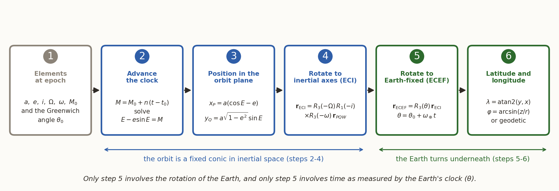
Step 1: the data. The six elements \((a,e,i,\Omega,\omega,M_0)\) at the epoch \(t_0\), and the Greenwich sidereal angle \(\theta_0\) at the epoch, from the sidereal-time formula of the time note.
Step 2: advance the clock. With \(M_0\) the mean anomaly at the epoch \(t_0\), the mean anomaly at time \(t\) is \(M=M_0+n(t-t_0)\), \(n=\sqrt{\mu/a^3}\), and Kepler’s equation \(E-e\sin E=M\) is solved for \(E\) (Newton’s method).
Step 3: position in the orbit plane (perifocal frame, \(\hat{\mathbf p}\) towards perigee): \[ x_P=a(\cos E-e),\qquad y_Q=a\sqrt{1-e^{2}}\,\sin E,\qquad z_W=0 . \tag{1}\]
Step 4: to inertial axes. Three rotations bring the orbit plane to its place: about the normal by \(\omega\) (perigee direction), about the line of nodes by \(i\) (tilt), about the polar axis by \(\Omega\) (node). With \(\mathbf R_1\) and \(\mathbf R_3\) the active rotation matrices of the perifocal note, which turn a vector by \(\theta\) about \(x\) and \(z\), \[ \mathbf r_{\rm ECI}=\mathbf R_3(\Omega)\,\mathbf R_1(i)\,\mathbf R_3(\omega)\,\mathbf r_{PQW},\qquad \mathbf R_3(\theta)=\begin{pmatrix}\cos\theta&-\sin\theta&0\\ \sin\theta&\cos\theta&0\\0&0&1\end{pmatrix},\quad \mathbf R_1(\theta)=\begin{pmatrix}1&0&0\\0&\cos\theta&-\sin\theta\\0&\sin\theta&\cos\theta\end{pmatrix}. \tag{2}\]
(Some books, Curtis among them, use passive matrices that rotate the frame instead; each is the transpose of the active one, \(R_3^{\rm passive}(\theta)=\mathbf R_3(-\theta)\), so the same product reads \(R_3(-\Omega)R_1(-i)R_3(-\omega)\) in their notation.)
Step 5: to Earth-fixed axes. The Earth-fixed frame is the inertial frame turned about the polar axis through the Greenwich angle \(\theta(t)=\theta_0+\omega_\oplus(t-t_0)\), with \(\omega_\oplus\) from the Earth’s rotation rate. A vector fixed in space therefore appears turned backwards by \(\theta\) in Earth-fixed components: \[ \mathbf r_{\rm ECEF}=\mathbf R_3\bigl(-\theta(t)\bigr)\,\mathbf r_{\rm ECI}. \tag{3}\]
Step 6: latitude and longitude. With \((x,y,z)=\mathbf r_{\rm ECEF}\) and \(r=|\mathbf r|\), the geocentric coordinates are \[ \lambda=\operatorname{atan2}(y,x),\qquad \varphi_{\rm gc}=\arcsin\frac zr . \tag{4}\] Maps and GPS use the geodetic latitude, measured from the local normal to the WGS-84 ellipsoid (flattening \(f_\oplus=1/298.257\)). It is obtained by a short fixed-point iteration, with \(p=\sqrt{x^2+y^2}\), \(e_E^2=f_\oplus(2-f_\oplus)\): \[ \varphi\leftarrow\operatorname{atan2}\!\left(z,\;p\Bigl(1-e_E^{2}\tfrac{N}{N+h}\Bigr)\right),\quad N=\frac{R_\oplus}{\sqrt{1-e_E^{2}\sin^{2}\varphi}},\quad h=\frac{p}{\cos\varphi}-N , \tag{5}\] started from \(\varphi=\operatorname{atan2}(z,\,p(1-e_E^2))\); six passes converge to well below a millimetre. The geodetic and geocentric latitudes differ by at most \(0.19^\circ\) (about \(21\) km on the ground), so for a picture at the scale of a continent either will do, but for pointing an antenna it matters.
The six steps are implemented in _gt.py, which draws every ground track in this note.
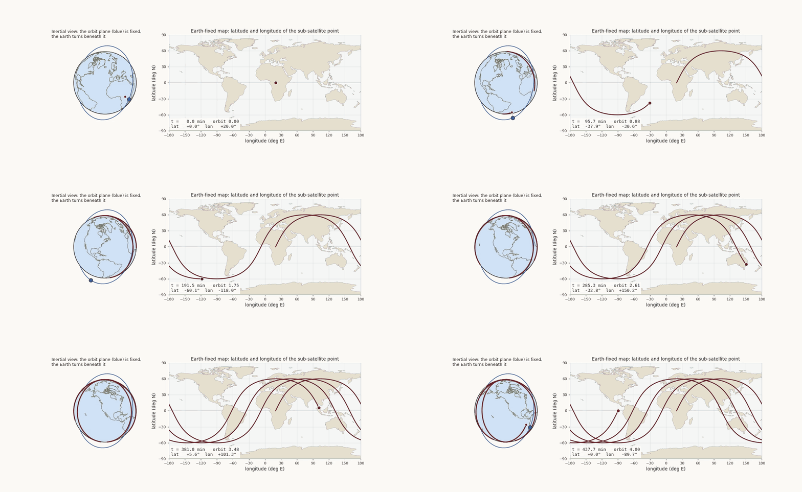
The animation shows the two views together for an orbit of \(60^\circ\) inclination and \(1200\) km altitude. On the left, the orbit plane (blue ring) does not move; the globe turns beneath it, and the red curve is painted on the rotating surface. On the right is the same curve on a map.
2.1 A closed form for circular orbits
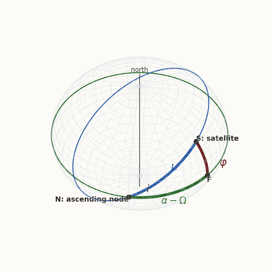
For a circular orbit (\(e=0\)) the six steps collapse into a formula that we can read. Use the argument of latitude \(u=\omega+f\) (the angle from the ascending node to the satellite, measured in the orbit plane). Steps 3 and 4 give the inertial unit vector \[ \hat{\mathbf r}_{\rm ECI}=\bigl(\cos\Omega\cos u-\sin\Omega\cos i\sin u,\ \ \sin\Omega\cos u+\cos\Omega\cos i\sin u,\ \ \sin i\sin u\bigr). \] The last component is \(\sin\varphi\) directly, and the first two can be combined as \(x+\mathrm iy=e^{\mathrm i\Omega}(\cos u+\mathrm i\cos i\sin u)\). Hence (Figure 3) \[ \boxed{\ \sin\varphi=\sin i\,\sin u,\qquad \tan(\alpha-\Omega)=\cos i\,\tan u,\qquad \lambda=\alpha-\theta(t)\ } \tag{6}\] where \(\alpha\) is the right ascension of the satellite. The first two relations are the standard relations of the right spherical triangle \(N\)–\(F\)–\(S\) of Figure 3 (hypotenuse \(u\), angle \(i\) at \(N\), sides \(\alpha-\Omega\) and \(\varphi\)). The third turns inertial right ascension into Earth-fixed longitude. Nothing in the derivation used \(e=0\): the three relations hold on any orbit, with \(u=\omega+f\). What is special about the circular orbit is only that \(u\) then grows uniformly in time, which is what the properties below use.
Reading Equation 6 gives the first properties of every circular ground track.
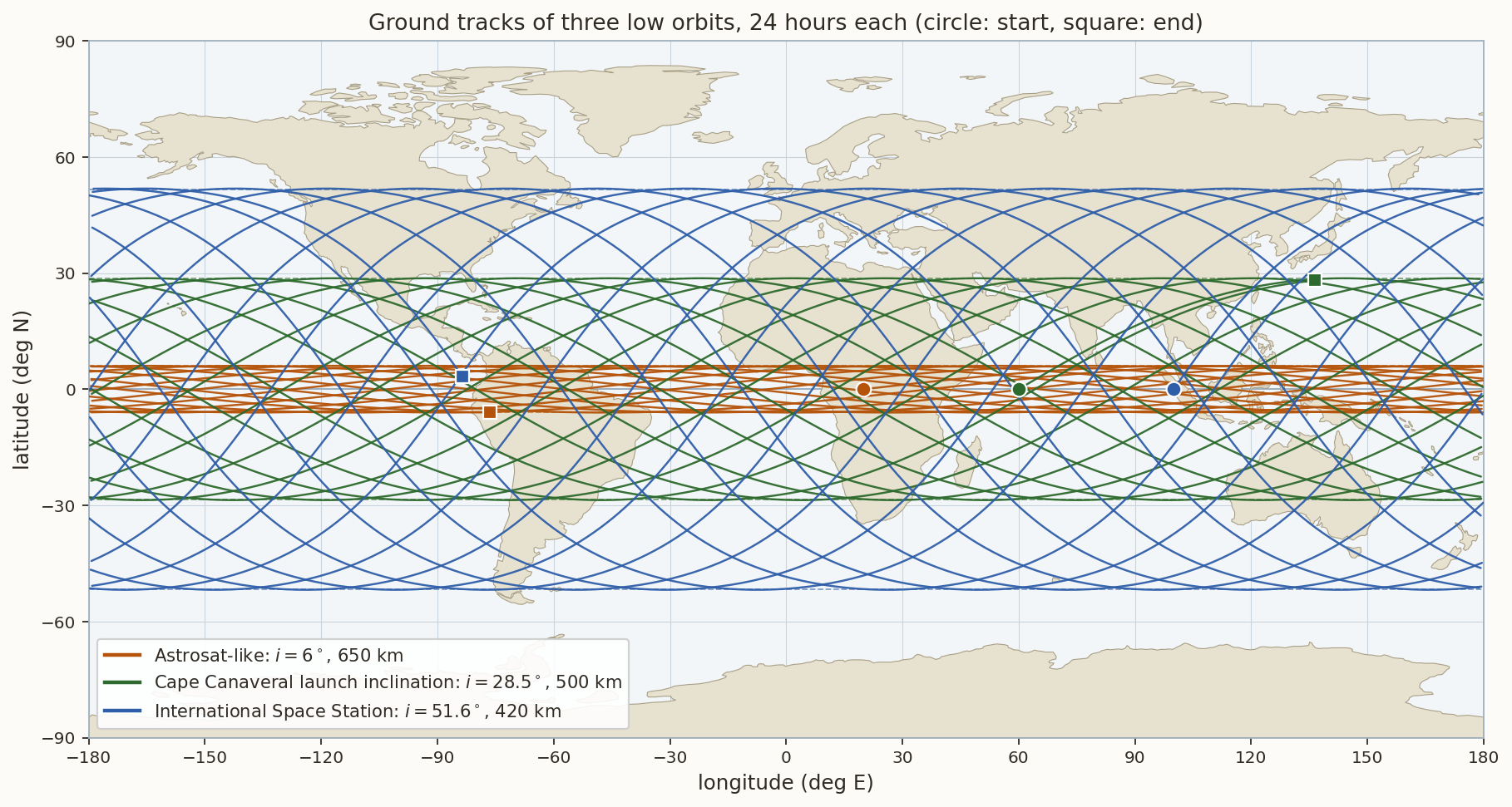
The largest latitude equals the inclination. \(\sin\varphi\le\sin i\), so \(|\varphi|_{\max}=i\) for \(i\le90^\circ\) and \(180^\circ-i\) for a retrograde orbit. The track lies between these parallels and touches them once per orbit (Figure 5, dashed lines). A polar orbit reaches the poles; an equatorial orbit never leaves the equator.
The track shifts west by \(\omega_\oplus T\) on every orbit. After one period \(u\) has increased by \(2\pi\) but \(\theta\) by \(\omega_\oplus T\), so the next equator crossing is displaced by \(-\omega_\oplus T\) in longitude: \[ \Delta\lambda_{\rm orbit}=-\omega_\oplus T=-360^\circ\frac{T}{T_{\rm sid}}\ \ (\text{with }J_2:\ -(\omega_\oplus-\dot\Omega)\,T_\Omega), \tag{7}\] where \(T_\Omega\) is the nodal period, the time between successive ascending nodes (defined precisely in Section 3.6). For \(T=92.97\) min (the ISS) this is \(23.3^\circ\), i.e. \(2594\) km at the equator; for a \(650\) km orbit \(24.5^\circ\) (\(2727\) km). The number of orbits per day is \(86\,400/T\): \(15.49\) for the ISS.
The heading at the equator is not the inclination. At the ascending node \(u=0\), \(\dot\varphi=n\sin i\) and \(\dot\lambda=n\cos i-\omega_\oplus\), so the track crosses the equator at an angle \(\beta\) (measured from east) with \[ \tan\beta=\frac{n\sin i}{n\cos i-\omega_\oplus}. \tag{8}\] For the ISS (\(\omega_\oplus/n=0.0647\), \(i=51.64^\circ\)) this gives \(\beta=54.7^\circ\), steeper than the inertial \(51.64^\circ\): the surface is moving eastward under the satellite. For a retrograde orbit the Earth’s rotation adds to the westward motion, and for a geostationary orbit (\(n=\omega_\oplus\), \(i=0\)) the numerator and the denominator both vanish and the track collapses to a point.
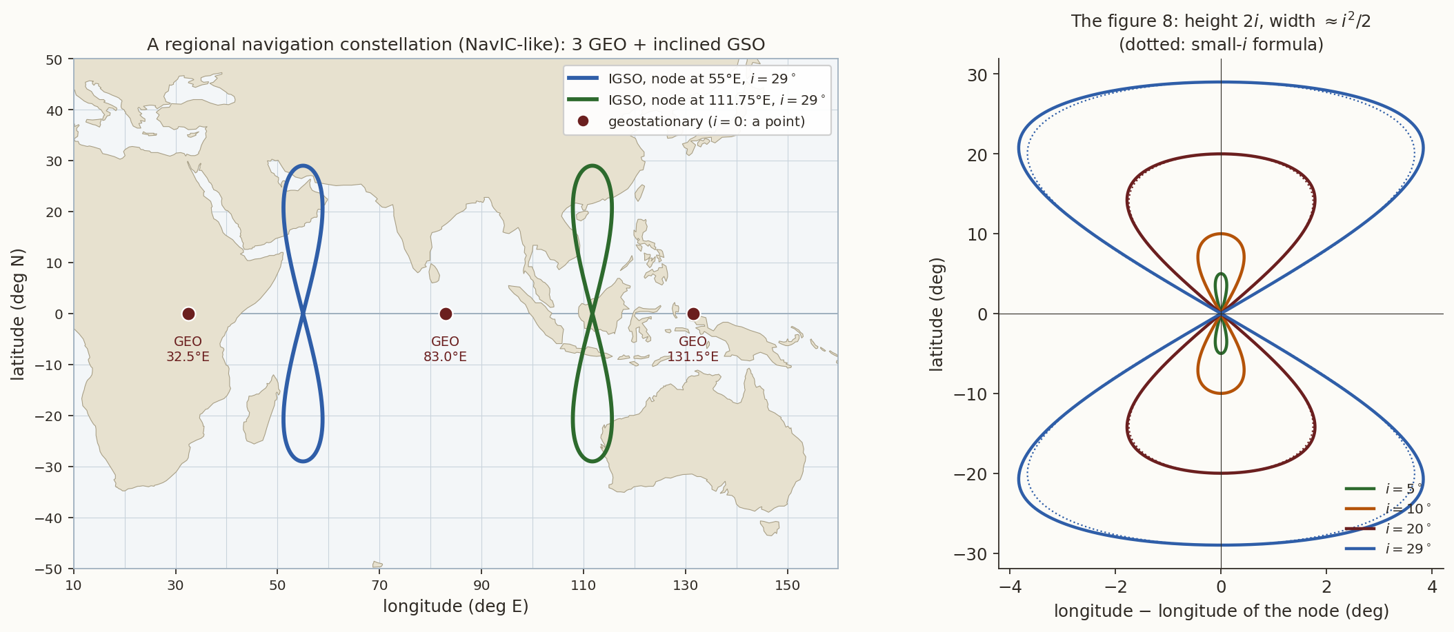
Small inclination at the geosynchronous radius gives a figure 8. If \(n=\omega_\oplus\) (the orbit is geosynchronous) then \(\lambda=\lambda_\Omega+\bigl[\operatorname{atan2}(\cos i\sin u,\cos u)-u\bigr]\), where \(\lambda_\Omega=\Omega-\theta+u\) is constant (because \(\dot u=\dot\theta\)) and is the geographic longitude of the node, and, for small \(i\), \(\operatorname{atan2}(\cos i\sin u,\cos u)-u\approx-\tfrac{i^2}{4}\sin2u\). The track is \[ \varphi=i\sin u,\qquad \lambda-\lambda_\Omega\approx-\frac{i^{2}}{4}\sin2u, \tag{9}\] a figure 8 of height \(2i\) and width \(i^2/2\), traversed once per sidereal day (Figure 8, right, dotted: Equation 9). For \(i=29^\circ\) the exact longitude excursion is \(\pm3.84^\circ\) and Equation 9 gives \(\pm3.67^\circ\); for \(i=10^\circ\), \(\pm0.439^\circ\) against \(\pm0.436^\circ\).
2.2 The effect of \(J_2\), and mean against osculating elements
Over many orbits the equatorial bulge (see Beyond the Point Mass) turns the orbit plane and rotates the perigee, and changes the mean motion. The secular rates, with \(p=a(1-e^2)\), are \[ \dot\Omega=-\tfrac32 nJ_2\Bigl(\frac{R_\oplus}{p}\Bigr)^{2}\cos i,\quad \dot\omega=\tfrac34 nJ_2\Bigl(\frac{R_\oplus}{p}\Bigr)^{2}(5\cos^2 i-1),\quad \dot M=n\Bigl[1+\tfrac34J_2\Bigl(\frac{R_\oplus}{p}\Bigr)^{2}\sqrt{1-e^2}\,(3\cos^2i-1)\Bigr]. \tag{10}\] To include \(J_2\) in the ground track, replace \(M\), \(\Omega\), \(\omega\) in steps 2 to 4 by \(M_0+\dot Mt\), \(\Omega_0+\dot\Omega t\), \(\omega_0+\dot\omega t\). The node drift changes Equation 7 as shown, and it is what makes sun-synchronous orbits possible (Section 3.3).
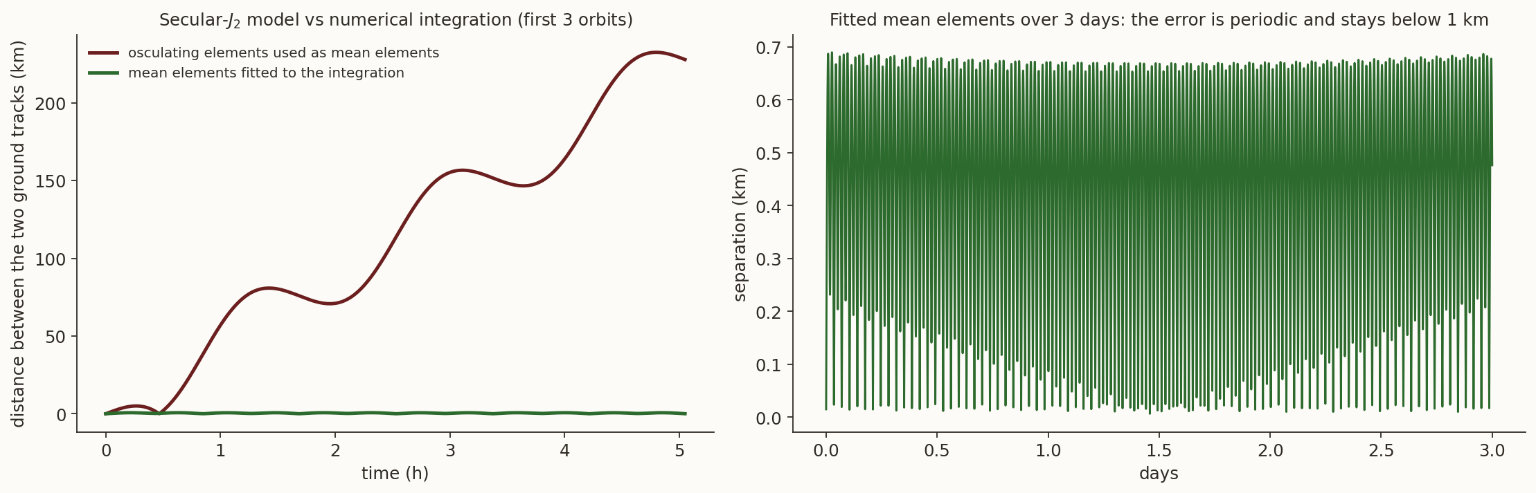
There is one trap. The rates of Equation 10 hold for mean elements: the elements averaged over an orbit. The osculating elements computed from an instantaneous position and velocity oscillate around them; in \(a\) the amplitude is about \(\tfrac32J_2R_\oplus^2/a\), roughly \(10\) km for a low orbit. Figure 4 makes the point. We integrated the equations of motion with the \(J_2\) acceleration for three days (DOP853, relative tolerance \(10^{-11}\)) for an \(800\) km orbit at \(i=98.6^\circ\), and compared with the analytic ground track. If the osculating elements at \(t=0\) are used as mean elements, the two tracks are \(76\) km apart after one orbit, \(1057\) km after a day and \(3256\) km after three days: the wrong semi-major axis (osculating \(7178.1\) km, mean \(7187.2\) km) makes the satellite run early. If the mean elements are fitted to the integration, the analytic track follows the integrated one to \(0.48\) km rms and \(0.69\) km at most over three days. The lesson is the standard one of mission analysis: use mean elements to describe orbits over long periods, and never mix them with osculating ones.
3 The standard ground tracks
3.1 Low Earth orbit
Figure 5 shows one day of three low orbits: a near-equatorial one (like India’s Astrosat, \(i=6^\circ\), \(650\) km), one at \(28.5^\circ\) (the latitude of Cape Canaveral, the lowest inclination reachable from there without a plane change), and the International Space Station (\(51.6^\circ\), \(420\) km). All three follow Equation 6: a sinusoid-like curve confined to the band \(|\varphi|\le i\), shifted west by \(23\) to \(25^\circ\) on every orbit. In a day the ISS completes \(15.5\) orbits, with successive tracks about \(2600\) km apart at the equator; over a few days it passes over every point between \(51.6^\circ\)N and \(51.6^\circ\)S, and it never sees the poles.
3.2 Polar orbit
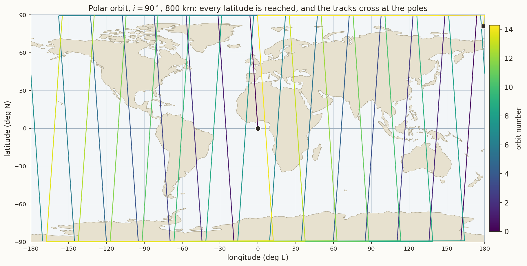
A polar orbit (\(i=90^\circ\)) passes over both poles on every revolution and, as the Earth turns underneath, eventually over every point on the globe (Figure 6). At \(800\) km the period is \(100.9\) min, there are \(14.3\) orbits per day, and successive tracks are \(25.3^\circ\) (\(2800\) km) apart at the equator. All tracks cross at the poles, so coverage is dense at high latitudes and sparsest at the equator. With \(J_2\) a polar orbit has \(\dot\Omega=0\): its plane stays fixed in inertial space, so relative to the Sun it turns once a year.
3.3 Sun-synchronous orbit
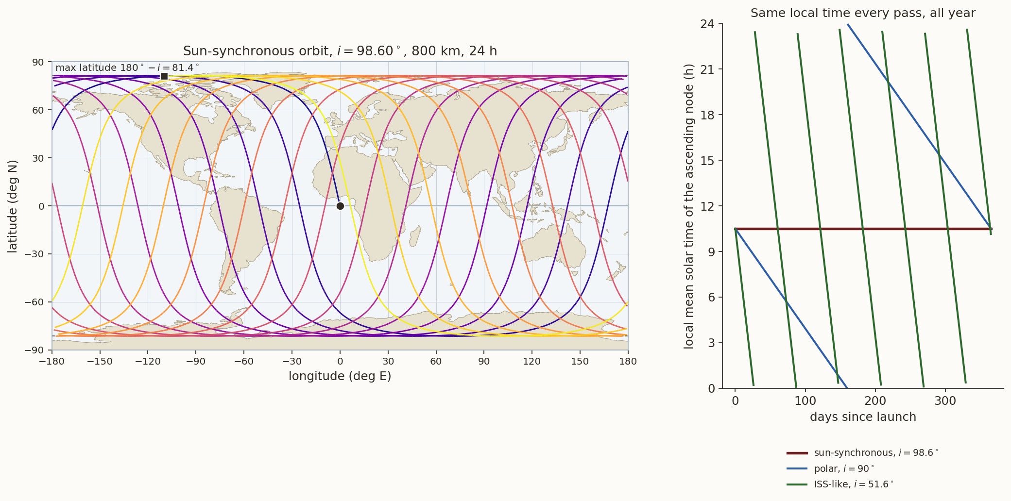
A sun-synchronous orbit (SSO) is not an orbit that follows the Sun. It is an orbit whose plane turns at exactly the rate at which the Sun’s right ascension increases, \[ \dot\Omega=\frac{2\pi}{365.2422\ \text{d}}=+0.98565^\circ/\text{day}, \tag{11}\] so that the angle between the orbit plane and the Earth–Sun line never changes. The satellite then crosses the equator at the same local mean solar time on every pass for the whole mission, which means the same sun elevation, the same shadow lengths and an unchanging power and thermal environment.
Equation 10 gives \(\dot\Omega\propto-\cos i\), and Equation 11 needs \(\dot\Omega>0\), so every sun-synchronous orbit is retrograde. Solving \(\dot\Omega=0.98565^\circ\)/day for the inclination gives, for circular orbits, \(i=98.60^\circ\) at \(800\) km and \(i=98.19^\circ\) at \(700\) km. The highest latitude is then \(180^\circ-i=81.4^\circ\), so an SSO covers the whole globe except for small polar caps. The right panel of Figure 7 shows the payoff: the local time of the ascending node stays constant for a year, whereas a polar orbit (fixed plane) drifts through \(24\) h in a year (\(-1.97\) h per \(30\) days) and the ISS orbit through \(24\) h in about two months, \(61\) days (\(-11.9\) h per \(30\) days).
History. The first Earth-observation satellite in a sun-synchronous orbit of the kind we use today was Landsat 1 (launched in 1972, then called ERTS-1; \(917\) km, \(99.1^\circ\)). Since then it has been the standard orbit for imaging, because the same local time gives comparable lighting from one pass to the next; a mid-morning descending node (about \(10{:}30\)) balances haze and shadows for optical imaging, a dawn-dusk orbit keeps the arrays in nearly continuous sunlight.
3.4 Geostationary and geosynchronous orbits
At \(a=42\,164\) km (\(T=\) one sidereal day) and \(i=0\) the sub-satellite point is fixed: the geostationary orbit is the only orbit whose ground track is a point. Its ground track is a single dot, and a single dot is exactly what a communications or weather satellite wants: a ground antenna does not have to move. At this altitude a satellite sees \(42\%\) of the surface (Section 5), so three satellites cover the equatorial and mid-latitude world.
If the same orbit is inclined (\(i>0\)) it is geosynchronous but no longer stationary: the sub-satellite point traces the figure 8 of Equation 9, once a day (Figure 8). India’s regional navigation system NavIC uses exactly this combination: three geostationary satellites (at \(32.5^\circ\)E, \(83^\circ\)E and \(131.5^\circ\)E) and four inclined geosynchronous ones (\(i=29^\circ\)) whose figures of eight are centred at \(55^\circ\)E and \(111.75^\circ\)E, so that at any moment several satellites are high in the sky over India. Historically, Syncom 2 (1963), the first geosynchronous satellite, had an inclination of \(33^\circ\) and drew a figure 8 before Syncom 3 (1964) became the first geostationary one.
3.5 Highly elliptical orbits: Molniya and Tundra
For \(e>0\) the satellite is not uniformly fast: by Kepler’s second law it lingers near apogee. The Molniya orbit (\(T=\) half a sidereal day, \(e=0.74\), \(a=26\,562\) km, perigee altitude \(528\) km, apogee altitude \(39\,840\) km) exploits this. Its inclination is \(i=63.4^\circ\), the critical inclination \(\arccos(1/\sqrt5)\) at which \(\dot\omega=0\) in Equation 10, so the apogee stays over the northern hemisphere instead of rotating away. The satellite is above \(55^\circ\)N for \(6.1\) h of each \(12\) h orbit, and the speed at perigee is \(6.7\) times that at apogee (Figure 9, dots are one hour apart). Two such orbits per day put apogee alternately over Russia (\(90^\circ\)E in the figure) and over North America. Geostationary satellites at high latitude are near the horizon; a Molniya satellite is almost overhead. The Tundra orbit (\(T\) = one sidereal day, \(e\approx0.27\), same inclination) gives a figure 8 with a small northern loop that dwells over one region for many hours.
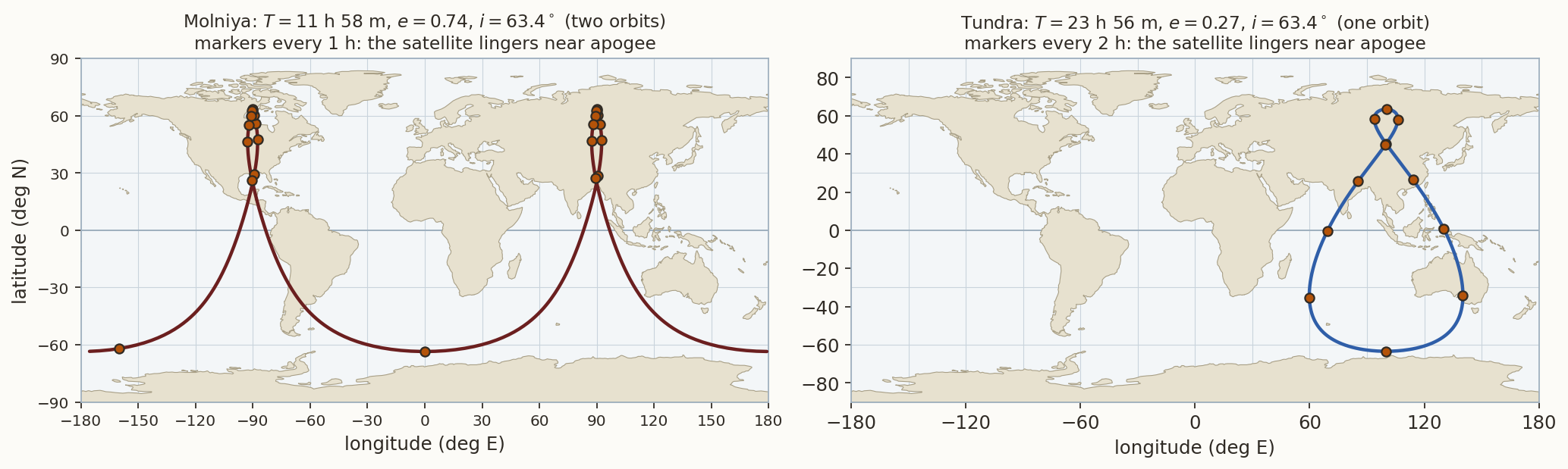
History. The first Molniya satellite was launched in April 1965. The reasoning was geometric: geostationary satellites are near the horizon at the high latitudes of the Soviet Union, and the highly elliptical orbit at the critical inclination is the cheapest way to stay high in the sky for most of the day.
3.6 Repeat ground tracks
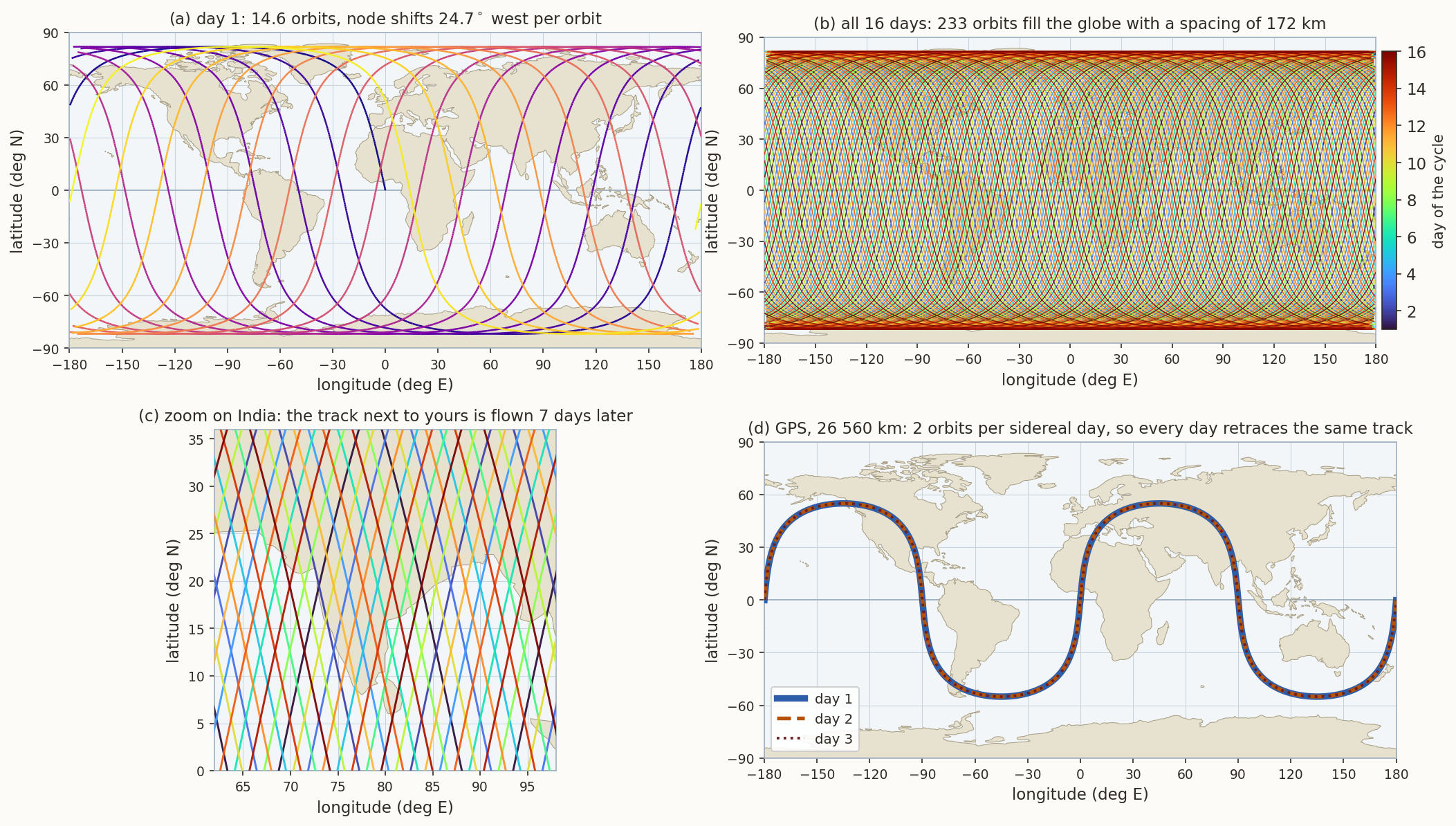
A ground track repeats if, after \(k\) revolutions, the Earth has turned through a whole number \(D\) of complete turns relative to the orbit plane. Between two successive ascending nodes, the Earth turns relative to the plane through \((\omega_\oplus-\dot\Omega)\,T_\Omega\), where \(T_\Omega=2\pi/\dot u\) is the nodal period (\(\dot u=\dot M+\dot\omega\) is the rate of the argument of latitude). Repeat after \(k\) orbits and \(D\) turns means \[ k\,(\omega_\oplus-\dot\Omega)\,T_\Omega=2\pi D \quad\Longleftrightarrow\quad \boxed{\ \frac{\dot M+\dot\omega}{\omega_\oplus-\dot\Omega}=\frac kD\ } \tag{12}\] with \(k\), \(D\) integers without common factor. With \(J_2\) neglected this reads \(n\,T_{\rm sid}=2\pi k/D\), i.e. \(T=(D/k)\,T_{\rm sid}\). The left-hand side of Equation 12 depends on \(a\) (and weakly on \(e\) and \(i\)), so for given \(k\), \(D\), \(i\), \(e\) it is solved for \(a\) by bisection. The ground track repeats after \(D\) nodal days, \(2\pi/(\omega_\oplus-\dot\Omega)\) each. For a sun-synchronous orbit \(\omega_\oplus-\dot\Omega\) is exactly \(2\pi\) per mean solar day, so the nodal day is the solar day (time note) and the cycle is \(D\) solar days; for a geosynchronous or GPS orbit \(\dot\Omega\) is tiny and the nodal day is very nearly the sidereal day.
After the cycle the \(k\) ascending nodes are equally spaced around the equator, \(360^\circ/k\) apart: the tracks fill in a grid with spacing \(2\pi R_\oplus/k\) at the equator. This is the design equation of an Earth-observation mission: choose \(k\) so that the spacing is a little less than the swath of the instrument.
We tested the solver against orbits whose parameters are published (Table 1): the agreement is a check on the whole chain of Equation 10 and Equation 12.
| Mission | \(k/D\) | Computed \(a-R_\oplus\) | Published |
|---|---|---|---|
| Sentinel-1 (SSO) | \(175/12\) | \(692.8\) km | \(693\) km |
| Sentinel-2 (SSO) | \(143/10\) | \(786.1\) km | \(786\) km |
| Resourcesat / IRS-1C (SSO) | \(341/24\) | \(817.0\) km | \(817\) km |
| Landsat 8, 9 (SSO) | \(233/16\) | \(699.6\) km | \(705\) km (osculating, at the equator) |
| Jason-3 (\(66.04^\circ\)) | \(127/10\) nodal days | \(1336.3\) km, cycle \(9.9156\) solar d | \(1336\) km, \(9.9156\) d |
| GPS (\(55^\circ\)) | \(2/1\) | \(20\,182.3\) km, \(a=26\,560.4\) km | \(a=26\,560\) km |
| Galileo (\(56^\circ\)) | \(17/10\) | \(a=29\,600.3\) km | \(a=29\,600\) km |
| GLONASS (\(64.8^\circ\)) | \(17/8\) | \(a=25\,507.6\) km | \(a=25\,508\) km |
The left panels of Figure 10 show the Landsat-like orbit. It flies \(14.56\) orbits per day, the ascending nodes advance \(24.72^\circ\) westward per orbit, and after \(16\) days the \(233\) tracks are spaced \(1.545^\circ=172.0\) km apart at the equator. The instrument swath of \(185\) km then gives a sidelap of \((185-172)/185=7\%\) at the equator, which grows toward the poles. Neighbouring tracks are flown seven days apart (modulo the \(16\)-day cycle), which is why a place is not re-imaged for a week after its neighbour. Panel (d) shows the case of GPS: two orbits per sidereal day, so that each day retraces the same path over the ground.
History. The altimetry satellite TOPEX/Poseidon (1992) was given a \(9.9156\)-day repeat cycle (\(127\) orbits) so that the tidal constituents, which are aliased by the sampling, appear at distinct periods (the lunar \(M_2\) tide is aliased to about \(62\) days) and can be separated from the slow sea-level changes that the mission was after. Jason-1, -2 and -3 fly the same ground track.
4 An interactive ground-track simulator
The figure below implements the six steps of Section 2 in JavaScript, in the browser. Pick a preset, or change the elements with the sliders (or type exact values into the boxes), and the ground track is redrawn. Press play to fly the satellite along its track with its footprint. Tick ground station to see the passes. The panel of read-outs gives the derived quantities of this note: period, nodal drift, shift per orbit, and, if the orbit repeats, the ratio of Equation 12.
Things to try (each takes a minute and each answers a question of this note).
- ISS. Play the preset for a day. How many orbits does it make? How far west does the track move on each orbit (read-out)? Compare with Equation 7.
- Geostationary, then increase \(i\) from \(0\) to \(29^\circ\) in small steps. Watch the point become a figure 8. Reproduce Equation 9.
- A 24-hour orbit. Set the preset “A 24-hour orbit”. The track is a straight line along the equator, running west at \(0.9856^\circ\)/day (time note, figure). Change \(a\) to \(42\,164.17\) km to stop it.
- Sun-synchronous. Take the SSO preset, untick \(J_2\): the node no longer moves and the local time of the pass is not constant. Tick it again and change \(i\) by \(0.5^\circ\): the read-out shows the drift \(\dot\Omega\) leaving \(0.9856^\circ\)/day.
- Repeat orbit. Press solve for a with \(k=233\), \(D=16\) (sun-synchronous ticked). Play the \(16\)-day cycle. Then type \(k=15\), \(D=1\) with the box unticked: an orbit with \(15\) revolutions per (nodal) day.
- Molniya. Set \(\omega=270^\circ\), then \(\omega=200^\circ\) and compare. Keep \(J_2\) ticked and change \(i\) from \(63.4^\circ\) to \(55^\circ\) or \(70^\circ\): the apogee drifts (\(\dot\omega\ne0\)) everywhere except at the critical inclination \(63.4^\circ\). (With \(J_2\) unticked the apogee never moves, at any inclination.)
- A station. Tick ground station at \((13.0^\circ\mathrm N,\,77.6^\circ\mathrm E)\) and read the passes of the SSO preset. Then move the station to Svalbard (\(78.2^\circ\)N, \(15.4^\circ\)E): how many passes per day now?
5 What ground tracks are used for
| Application | Orbit | Ground-track property used | Example |
|---|---|---|---|
| Optical / radar Earth observation | sun-synchronous, repeat orbit | same local time every pass; global coverage; track spacing \(<\) swath | Landsat, Sentinel, Resourcesat |
| Altimetry | non-sun-synchronous, exact repeat | repeat cycle with aliasing of tides | TOPEX/Poseidon, Jason |
| Continuous regional service | geostationary | fixed sub-satellite point | INSAT, GOES, Meteosat |
| Regional navigation | GEO + inclined geosynchronous | figure 8 over the region | NavIC, QZSS, BeiDou |
| High-latitude communication | Molniya, Tundra | slow near apogee over the north | Molniya, Sirius XM |
| Global navigation | MEO, repeat every few days | track repeats every sidereal day (GPS), every 8–10 days (GLONASS, Galileo) | GPS, Galileo |
| Weather, global | polar / SSO | all latitudes, twice a day | Metop, NOAA |
| Crew and cargo | ISS, \(51.6^\circ\) | visible from most populated latitudes; launch from mid-latitude sites | ISS |
5.1 Coverage: footprints and swaths
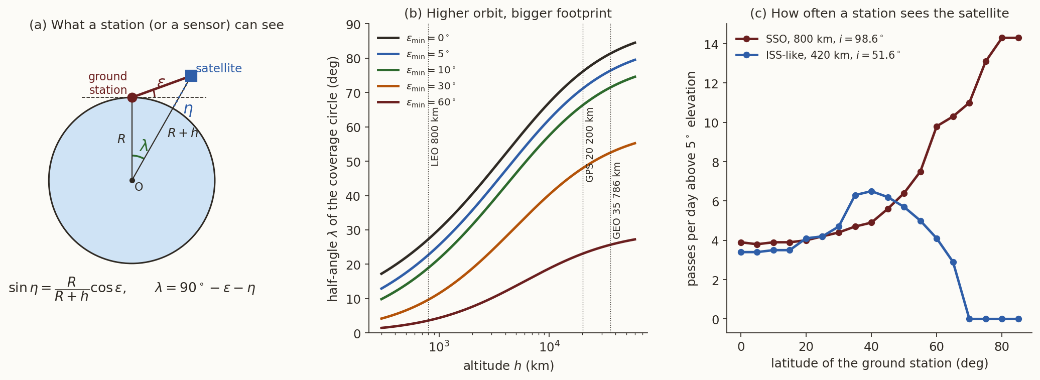
A satellite at altitude \(h\) sees, above a minimum elevation angle \(\varepsilon\) (in this section \(\varepsilon\) is an elevation), a circle on the ground of angular radius \(\psi\) (the Earth central angle) around the sub-satellite point (Figure 12, left). From the triangle Earth centre–station–satellite, \[ \sin\eta=\frac{R_\oplus}{R_\oplus+h}\cos\varepsilon,\qquad \psi=90^\circ-\varepsilon-\eta , \tag{13}\] where \(\eta\) is the nadir angle at which the station is seen from the satellite. At \(800\) km with \(\varepsilon=10^\circ\) the coverage radius is \(\psi=18.95^\circ\) (\(2109\) km); at \(\varepsilon=0\) it is \(27.3^\circ\). For a geostationary satellite \(\psi=81.3^\circ\) at \(\varepsilon=0\): it sees \(\tfrac12(1-\cos81.3^\circ)=42.4\%\) of the whole surface. Three of them, \(120^\circ\) apart, cover all longitudes up to a latitude of about \(\pm72^\circ\) at \(\varepsilon=0\), and about \(\pm62^\circ\) if \(5^\circ\) of elevation is required. For an imaging satellite the footprint is the instrument swath, about \(100\) to \(200\) km, and the ground track is its centre line: the design condition is the spacing of the repeat grid (Equation 12) against the swath.
5.2 Ground stations: how often, and for how long
The same equation gives the contact with a ground station: the satellite is visible when its sub-satellite point is within \(\psi\) of the station (Figure 12, right; the dashed circle in the simulator). We counted passes above \(5^\circ\) elevation over ten days by direct computation (Table 3).
| Station | SSO \(800\) km: passes/day | contact min/day | min per pass | ISS: passes/day | contact min/day |
|---|---|---|---|---|---|
| Equator | \(3.9\) | \(37\) | \(9.5\) | \(3.4\) | \(23\) |
| Thiruvananthapuram (\(8.5^\circ\)N) | \(3.7\) | \(37\) | \(10.0\) | \(3.6\) | \(23\) |
| Bengaluru (\(13.0^\circ\)N) | \(3.8\) | \(37\) | \(9.8\) | \(3.6\) | \(24\) |
| Delhi (\(28.6^\circ\)N) | \(4.3\) | \(42\) | \(9.8\) | \(4.6\) | \(30\) |
| Svalbard (\(78.2^\circ\)N) | \(14.3\) | \(156\) | \(10.9\) | \(0\) | \(0\) |
A polar-type orbit passes near the poles on every one of its \(14.3\) orbits per day, so a station at \(78^\circ\)N is in contact on every orbit: this is why polar-orbit missions use high-latitude stations for data download. A station at low latitude sees such a satellite only three to four times a day, each pass lasting about ten minutes. The ISS never rises above \(5^\circ\) from Svalbard. Two practical numbers follow: a low-latitude station can download a few tens of minutes of data per day from a polar LEO satellite (which is why on-board storage and a high-latitude station matter), and a low-inclination LEO satellite is best served by stations near its maximum latitude.
5.3 The launch site sets the lowest inclination
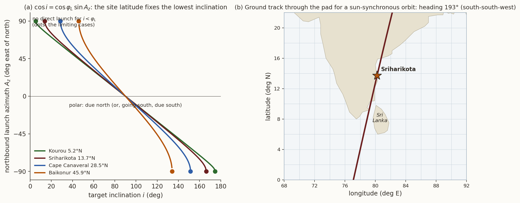
A launch vehicle can put a satellite directly into an orbit of inclination \(i\) only if \(i\ge\varphi_L\), the latitude of the launch site, because the orbit plane contains the Earth’s centre and the launch point, so it reaches at least latitude \(\varphi_L\). The launch azimuth \(A_z\) (from north, inertial) follows from the spherical triangle of Figure 3 applied to the launch point: \[ \cos i=\cos\varphi_L\,\sin A_z . \tag{14}\] A due-east launch (\(A_z=90^\circ\)) gives \(i=\varphi_L\) and also takes full advantage of the Earth’s rotation, which contributes \(\omega_\oplus R_\oplus\cos\varphi_L\) to the speed: \(463\) m/s at Kourou (\(5.2^\circ\)N), \(452\) m/s at Sriharikota (\(13.7^\circ\)N), \(409\) m/s at Cape Canaveral (\(28.5^\circ\)N), \(324\) m/s at Baikonur (\(45.9^\circ\)N). For a sun-synchronous orbit with \(i=98.7^\circ\) from Sriharikota, Equation 14 gives \(A_z\approx-9^\circ\) or \(189^\circ\): the vehicle flies almost due south, against the rotation of the Earth, and the ground track through the launch site heads \(193^\circ\), south-south-west, after the rotation of the Earth is taken out (Figure 13, right). This track passes close to the west coast of Sri Lanka, and avoiding an overflight of Sri Lanka is the reason usually given for the dog-leg manoeuvre that India’s PSLV flies on its sun-synchronous launches (the ascent path, unlike the final orbit’s track, is bent around the island; our figure shows only the orbit’s ground track through the pad).
Summary and outlook
In one paragraph. The ground track is the inertial orbit seen from the rotating Earth: elements \(\to\) Kepler \(\to\) perifocal \(\to\) inertial \(\to\) rotate by \(\theta=\theta_0+\omega_\oplus t\) \(\to\) \((\varphi,\lambda)\). For circular orbits \(\sin\varphi=\sin i\sin u\) and \(\tan(\alpha-\Omega)=\cos i\tan u\): the highest latitude is \(i\), the track moves \(360^\circ\,T/T_{\rm sid}\) west per orbit, and near the geosynchronous radius a small inclination gives a figure 8 of width \(i^2/2\). \(J_2\) adds \(\dot\Omega\), \(\dot\omega\), \(\dot M\) (use mean elements!) and makes sun-synchronous orbits possible; the repeat condition is \((\dot M+\dot\omega)/(\omega_\oplus-\dot\Omega)=k/D\). Every application in Table 2 is a statement about one of these properties.
The numbers that follow from formulas in this note are checked by ground-tracks-verify.py.
What we left out. (i) Precession, nutation and polar motion. The transformation from ECI to ECEF is here a single rotation. The full IAU 2006/2000A transformation adds precession, nutation and polar motion, which move points on the ground by up to a few hundred metres. (ii) Drag and other perturbations, which change \(a\) and hence the period and the repeat pattern: repeat-orbit missions carry propellant to hold the ground track within a tolerance band (typically \(\pm1\) km of the reference track for the Landsat series; check the mission documentation).
Further reading. H. D. Curtis, Orbital Mechanics for Engineering Students (ground tracks); D. A. Vallado, Fundamentals of Astrodynamics and Applications (ground tracks and repeat orbits, coverage).
Exercises
- Heading at the node. Evaluate Equation 8 for the ISS (\(T=92.97\) min, \(i=51.64^\circ\)). What is the heading for an SSO at \(800\) km? Why is it larger than \(90^\circ\)? (Answers: \(54.7^\circ\); \(102.5^\circ\), because the orbit is retrograde and the Earth’s rotation adds to the westward motion.)
- SSO design. Find the inclination of a circular sun-synchronous orbit at \(700\) km from \(\dot\Omega=0.9856^\circ\)/day. (Answer: \(98.19^\circ\).)
- Track spacing. For \(233\) orbits in \(16\) days, find the equatorial spacing of tracks in degrees and kilometres, and the sidelap of a \(185\) km swath. (Answers: \(1.545^\circ\), \(172\) km, \(7\%\).)
- Repeat orbit, no \(J_2\). Find the altitude of a circular orbit with \(15\) revolutions in one stellar day, neglecting \(J_2\). (Answer: about \(554\) km.)
- Figure 8. For a geosynchronous orbit with \(i=29^\circ\) find the width and height of the figure 8 from Equation 9, and compare with the exact value \(\pm3.84^\circ\) of the longitude excursion.
- Footprint. At what altitude does a satellite see an Earth central angle of \(\psi=30^\circ\) at \(\varepsilon=10^\circ\)? Use Equation 13. (Answer: \(\eta=50^\circ\), \(R_\oplus+h=R_\oplus\cos10^\circ/\sin50^\circ\), \(h\approx1820\) km.)
- Launch. Which is the lowest inclination reachable directly from Kourou? From Baikonur? What is the northbound launch azimuth from Sriharikota into a \(98.6^\circ\) orbit? (Answers: \(5.2^\circ\); \(45.9^\circ\); \(-8.9^\circ\), i.e. \(351.1^\circ\).)
- Simulator. Using Section 4, find the altitude and inclination of a sun-synchronous orbit that repeats after \(D=16\) solar days with \(k=229\) orbits, and read off the spacing of the tracks (\(360^\circ/229=1.572^\circ\)). Why would \(k=232\), \(D=16\) not be a good choice? (Hint: \(\gcd(232,16)=8\).) (Answers: \(a=7160.1\) km, altitude \(781.9\) km, \(i=98.53^\circ\), spacing \(175\) km; \(232/16=29/2\) repeats after \(2\) days, not \(16\).)