Patched Conics
The sphere of influence, Laplace’s radius, and flying between worlds with one two-body problem at a time
1 Where we are going
A spacecraft that leaves the Earth for Mars is pulled by the Sun, the Earth, Mars, the Moon, Jupiter and everything else, all the time. Its motion is an \(n\)-body problem, and the \(n\)-body problem has no closed-form solution. Yet mission designers size the propellant tank of a Mars probe, choose its launch date and decide where its engine must fire, with nothing more than a calculator and the two-body formulas of the first half of this course.
They can do this because, at almost every moment of the journey, one body dominates. Near the Earth, the Earth’s pull decides the motion and the Sun’s is a small correction; far from every planet, the Sun decides it. The patched-conic method takes this literally. It splits the journey into pieces, treats each piece as a two-body problem about the body that dominates there, and joins (patches) the pieces end to end. Each piece is a conic, hence the name.
The method needs one new idea: a rule for deciding where one body stops dominating and the next takes over. That rule is the sphere of influence, and most of the physics of this note is in deriving it.
When you finish, you should be able to answer all of the following without hand-waving.
- Why is the boundary between the Earth’s region and the Sun’s region not where their pulls are equal?
- Where does the formula \(r_{\rm SOI}=R\,(m/M)^{2/5}\) come from, and how wrong is it?
- What exactly is patched at the boundary: position, velocity, energy?
- How do you turn a heliocentric transfer into a \(\Delta v\) from a parking orbit, and where must the engine fire?
- How does a planetary flyby change a spacecraft’s heliocentric speed, when its speed relative to the planet does not change at all?
- What changes when the target is out of the plane: why does a launch site’s latitude limit the departure, and why is a \(180^\circ\) transfer between two inclined orbits a disaster?
- How good is the answer, compared with integrating the real equations of motion?
The note is in three stages. Section 2 to Section 4 build the tools: the prerequisites, and the sphere of influence. Section 5 states the method, and Section 6 and Section 7 work six examples with it, three in a plane and three out of it. Section 8 then checks the method against numerical integration.
2 What you need first
Everything in this note rests on the two-body problem. This section collects the results we will use, with short derivations, so that the rest of the note can use them without stopping. If you are comfortable with them, skim the boxed summary at the end.
2.1 The two-body problem
A small body moving about a much larger one of gravitational parameter \(\mu=GM\) obeys
\[ \ddot{\mathbf r}=-\frac{\mu}{r^3}\,\mathbf r . \tag{1}\]
Two quantities are conserved: the specific angular momentum \(\mathbf h=\mathbf r\times\dot{\mathbf r}\) and the specific energy
\[ \varepsilon=\frac{v^2}{2}-\frac{\mu}{r}=-\frac{\mu}{2a}. \tag{2}\]
The second form, with \(a\) the semi-major axis, is the vis-viva law; solved for the speed, \(v^2=\mu\,(2/r-1/a)\). The orbit is a conic \(r=p/(1+e\cos f)\), with \(p=h^2/\mu\) and \(f\) the true anomaly. Its type is set by the sign of \(\varepsilon\):
| \(\varepsilon\) | \(a\) | \(e\) | orbit |
|---|---|---|---|
| \(<0\) | \(>0\) | \(<1\) | ellipse (circle if \(e=0\)) |
| \(0\) | \(\infty\) | \(1\) | parabola |
| \(>0\) | \(<0\) | \(>1\) | hyperbola |
We use the convention of the Two-body Problem deck that \(a<0\) for a hyperbola, so that \(\varepsilon=-\mu/2a\) holds for all three.
2.2 The hyperbola, in the variables we will need
Every arrival at, or departure from, a planet in this note is a hyperbola about that planet. The hyperbola is usually described by \(a\) and \(e\), but the quantities a mission designer is given are different: how fast the spacecraft approaches from far away, and how close it should pass. So we rewrite the hyperbola in those terms.
Excess speed. Far from the planet, \(r\to\infty\) and Equation 2 gives \(\varepsilon=v_\infty^2/2\). The speed \(v_\infty\) that remains “at infinity” is the hyperbolic excess speed. Comparing with \(\varepsilon=-\mu/2a\):
\[ v_\infty^2=-\frac{\mu}{a},\qquad\text{i.e.}\qquad |a|=\frac{\mu}{v_\infty^2}. \tag{3}\]
Periapsis. The closest approach is \(r_p=a(1-e)=|a|(e-1)\). Given \(v_\infty\) and \(r_p\), this fixes the eccentricity:
\[ e=1+\frac{r_p}{|a|}=1+\frac{r_p\,v_\infty^2}{\mu}. \tag{4}\]
Speed at periapsis. By vis-viva with \(a=-\mu/v_\infty^2\),
\[ v_p^2=\mu\Bigl(\frac{2}{r_p}+\frac{v_\infty^2}{\mu}\Bigr)=v_\infty^2+\frac{2\mu}{r_p}=v_\infty^2+v_{\rm esc}^2(r_p). \tag{5}\]
The speed at periapsis is the excess speed and the local escape speed added in quadrature.
Directions of the asymptotes. As \(r\to\infty\) the orbit equation needs \(1+e\cos f\to0\), so the true anomaly tends to
\[ f_\infty=\arccos\Bigl(-\frac1e\Bigr),\qquad 90^\circ<f_\infty<180^\circ . \tag{6}\]
The incoming asymptote is at \(-f_\infty\), the outgoing one at \(+f_\infty\).
Turning angle. Between the incoming and outgoing asymptotes the velocity relative to the planet turns through \(\delta=2f_\infty-180^\circ\). With \(\cos f_\infty=-1/e\) this simplifies: \(\sin(\delta/2)=\sin(f_\infty-90^\circ)=-\cos f_\infty=1/e\), so
\[ \delta=2\arcsin\frac1e . \tag{7}\]
A close, slow pass (large \(\mu\), small \(r_p\), small \(v_\infty\)) has \(e\) near \(1\) and turns the velocity by nearly \(180^\circ\); a distant, fast pass hardly turns it at all.
Impact parameter. Far away, the incoming path is a straight line that would miss the planet by a distance \(b\), the impact parameter or aim radius. There the velocity is \(v_\infty\) and is perpendicular to the miss distance, so \(h=b\,v_\infty\). At periapsis \(h=r_pv_p\). Equating, and using Equation 5,
\[ b=\frac{r_pv_p}{v_\infty}=r_p\sqrt{1+\frac{2\mu}{r_p v_\infty^2}} . \tag{8}\]
\(b\) is always larger than \(r_p\): gravity bends the path inwards, so the spacecraft must be aimed wide of the periapsis it will actually reach. This is gravitational focusing.
2.3 A burn at periapsis
Leaving a circular parking orbit of radius \(r_p\) on a hyperbola of excess speed \(v_\infty\) is best done with one tangential burn at the periapsis of the hyperbola, which is then a point of the parking orbit. From Equation 5, the burn is
\[ \Delta v=\sqrt{v_\infty^2+\frac{2\mu}{r_p}}-\sqrt{\frac{\mu}{r_p}} . \tag{9}\]
Capture is the same burn, run backwards. Why at periapsis? A small burn there changes the energy by \(\Delta\varepsilon\approx v\,\Delta v\), and \(v\) is largest at periapsis: the Oberth effect of the Orbital Maneuvers deck.
2.4 The Hohmann transfer
Between circular orbits of radii \(r_1<r_2\) about a body \(\mu\), the Hohmann ellipse has \(a_t=(r_1+r_2)/2\). Vis-viva gives its speeds at the two apsides, and the time is half its period:
\[ V_{t1}=\sqrt{\mu\Bigl(\frac2{r_1}-\frac1{a_t}\Bigr)},\qquad V_{t2}=\sqrt{\mu\Bigl(\frac2{r_2}-\frac1{a_t}\Bigr)},\qquad t_{12}=\pi\sqrt{\frac{a_t^3}{\mu}} . \tag{10}\]
2.5 Frames that move
We will describe one spacecraft in two frames: one centred on the Sun, one centred on a planet. Both frames keep their axes parallel to the same fixed directions; the planet frame simply moves with the planet. For two such frames, positions and velocities add:
\[ \mathbf R_{\rm s/c}=\mathbf R_{\rm planet}+\mathbf r,\qquad \mathbf V_{\rm s/c}=\mathbf V_{\rm planet}+\mathbf v . \tag{11}\]
Convention for this note. Capital letters (\(\mathbf R\), \(\mathbf V\)) are heliocentric; small letters (\(\mathbf r\), \(\mathbf v\)) are relative to a planet. So \(\mathbf v_\infty=\mathbf V_{\rm s/c}-\mathbf V_{\rm planet}\) is the spacecraft’s velocity relative to the planet, far from it.
2.6 Phase angle and synodic period
A Hohmann transfer only works if the target planet is at the arrival point when the spacecraft gets there. During the flight time \(t_{12}\) the target moves through \(n_2t_{12}\), with \(n_2\) its mean motion. It must therefore lead the departure planet at launch by the phase angle
\[ \phi_0=180^\circ-n_2\,t_{12}. \tag{12}\]
The relative angle of two planets repeats after the synodic period \(S\). Planet 1 gains on planet 2 at the rate \(n_1-n_2\), and a full lap of \(360^\circ\) takes
\[ S=\frac{2\pi}{|n_1-n_2|}=\frac{1}{|1/T_1-1/T_2|} . \tag{13}\]
What we will use. \(v_\infty^2=-\mu/a\); \(e=1+r_pv_\infty^2/\mu\); \(v_p^2=v_\infty^2+2\mu/r_p\); \(\cos f_\infty=-1/e\); \(\delta=2\arcsin(1/e)\); \(b=r_p\sqrt{1+2\mu/(r_pv_\infty^2)}\); the Hohmann speeds and time; \(\mathbf v=\mathbf V-\mathbf V_{\rm planet}\); the phase angle and the synodic period.
3 Why one body at a time?
Consider a spacecraft just leaving the Earth, at a few Earth radii. The Earth pulls it with \(\mu_\oplus/r^2\), a few m/s\(^2\). The Sun pulls it with about \(\mu_\odot/(1\,{\rm AU})^2=5.93\ \mathrm{mm/s^2}\), a thousand times less. But the Sun also pulls the Earth with almost the same acceleration, so in a frame moving with the Earth the Sun’s effect nearly cancels. What survives is the difference between the Sun’s pull on the spacecraft and on the Earth: the tidal acceleration, which is smaller still.
Now go far from the Earth, half way to Mars, about \(0.6\) AU from the Earth and \(1.26\) AU from the Sun. The Earth’s pull has fallen to about \(0.05\ \mu\mathrm{m/s^2}\), and the Sun’s is about \(3.7\ \mathrm{mm/s^2}\), nearly a hundred thousand times larger. Here it is natural to measure the motion from the Sun, and to treat the Earth’s pull as the small correction.
So the same spacecraft, in the same gravitational field, is best described relative to the Earth in one region and relative to the Sun in another. Somewhere in between there must be a boundary. The question is where, and by what criterion.
4 The sphere of influence
4.1 A first guess, and why it fails
The obvious guess is the distance at which the two pulls are equal. Measure \(r\) from the planet (mass \(m\)) along the line to the Sun (mass \(M\), at distance \(R\) from the planet). The pulls are equal when
\[ \frac{Gm}{r^2}=\frac{GM}{(R-r)^2}\quad\Longrightarrow\quad \frac{R-r}{r}=\sqrt{\frac Mm} \quad\Longrightarrow\quad r=\frac{R\sqrt{m/M}}{1+\sqrt{m/M}} . \]
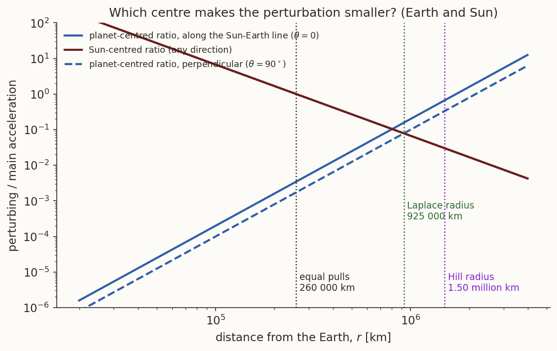
For the Earth, \(m/M=\mu_\oplus/\mu_\odot=3.0035\times10^{-6}\) and \(r\approx259\,000\) km.
This cannot be right. The Moon is at \(384\,400\) km, well outside that distance: the Sun pulls the Moon about twice as hard as the Earth does. Yet the Moon goes round the Earth, not round the Sun on an independent orbit. The guess fails because it compares the wrong things. What decides whether the Earth is a good centre is not the size of the Sun’s pull, but how much that pull disturbs the motion relative to the Earth. And a pull that acts almost equally on the Earth and on the Moon hardly disturbs their relative motion at all.
4.2 Two descriptions of the same motion
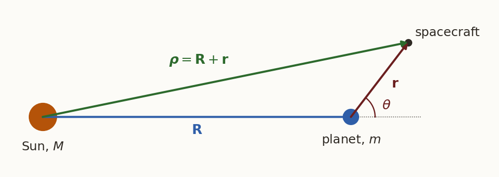
Let us make this precise. Three bodies (Figure 1): the Sun (mass \(M\)), a planet (mass \(m\)) and a spacecraft whose own mass is negligible. Call
- \(\mathbf R\) the planet’s position relative to the Sun,
- \(\mathbf r\) the spacecraft’s position relative to the planet,
- \(\boldsymbol\rho=\mathbf R+\mathbf r\) the spacecraft’s position relative to the Sun,
and \(\theta\) the angle between \(\mathbf r\) and the Sun–planet line.
In an inertial frame, with positions \(\mathbf X_{\odot}\), \(\mathbf X_p\), \(\mathbf X_s\), Newton’s law gives each body’s acceleration. The spacecraft is pulled by both; the planet is pulled by the Sun; the Sun is pulled by the planet (the spacecraft is too light to pull anything):
\[ \ddot{\mathbf X}_s=-\frac{GM}{\rho^3}\boldsymbol\rho-\frac{Gm}{r^3}\mathbf r,\qquad \ddot{\mathbf X}_p=-\frac{GM}{R^3}\mathbf R,\qquad \ddot{\mathbf X}_\odot=+\frac{Gm}{R^3}\mathbf R . \]
Relative to the planet. \(\mathbf r=\mathbf X_s-\mathbf X_p\), so \(\ddot{\mathbf r}=\ddot{\mathbf X}_s-\ddot{\mathbf X}_p\):
\[ \ddot{\mathbf r}=\underbrace{-\frac{Gm}{r^3}\mathbf r}_{\text{main: the planet}} \;\underbrace{-\,GM\Bigl(\frac{\boldsymbol\rho}{\rho^3}-\frac{\mathbf R}{R^3}\Bigr)}_{\text{perturbation: the Sun}} . \tag{14}\]
The Sun’s contribution is the difference between its pull on the spacecraft (\(\boldsymbol\rho/\rho^3\)) and its pull on the planet (\(\mathbf R/R^3\)), exactly as argued in words.
Relative to the Sun. \(\boldsymbol\rho=\mathbf X_s-\mathbf X_\odot\), so \(\ddot{\boldsymbol\rho}=\ddot{\mathbf X}_s-\ddot{\mathbf X}_\odot\):
\[ \ddot{\boldsymbol\rho}=\underbrace{-\frac{GM}{\rho^3}\boldsymbol\rho}_{\text{main: the Sun}} \;\underbrace{-\,Gm\Bigl(\frac{\mathbf r}{r^3}+\frac{\mathbf R}{R^3}\Bigr)}_{\text{perturbation: the planet}} . \tag{15}\]
The second perturbing term, \(\mathbf R/R^3\), is there because the Sun itself is being accelerated by the planet: the “indirect” term.
Both equations are exact, and they describe the same motion. Each is a two-body problem plus a perturbation. If we must throw one perturbation away (that is what the patched-conic method does), we should use the description in which the perturbation is relatively smaller.
To compare the two we need sizes, so give the two parts of each equation names. Write Equation 14 and Equation 15 as
\[ \ddot{\mathbf r}=\mathbf a_{\rm planet}+\mathbf p_{\rm planet},\qquad \ddot{\boldsymbol\rho}=\mathbf a_{\rm Sun}+\mathbf p_{\rm Sun}, \]
where \(\mathbf a\) is the main (two-body) acceleration and \(\mathbf p\) the perturbing acceleration, the underbraced terms. Both are vectors. Laplace’s comparison uses only their lengths, which we denote by capitals:
\[ A=|\mathbf a|,\qquad P=|\mathbf p| . \]
So \(P_{\rm planet}\), for instance, is a scalar: the magnitude of the Sun’s perturbing acceleration when the motion is measured from the planet.
4.3 The two perturbations, near the planet
Near the planet, \(r\ll R\). We now find the leading term of each perturbation in the small ratio \(r/R\).
The Sun’s tidal term, in Equation 14. We need \(\boldsymbol\rho/\rho^3\) with \(\boldsymbol\rho=\mathbf R+\mathbf r\). First the magnitude:
\[ \rho^2=R^2+2\,\mathbf R\cdot\mathbf r+r^2=R^2\Bigl(1+\frac{2\,\hat{\mathbf R}\cdot\mathbf r}{R}+\frac{r^2}{R^2}\Bigr). \]
Raise to the power \(-3/2\) and keep terms of first order in \(r/R\), using \((1+x)^{-3/2}\approx1-\tfrac32x\):
\[ \frac1{\rho^3}=\frac1{R^3}\Bigl(1-\frac{3\,\hat{\mathbf R}\cdot\mathbf r}{R}+O\bigl(r^2/R^2\bigr)\Bigr). \]
Now multiply by \(\boldsymbol\rho=\mathbf R+\mathbf r\), term by term, writing \(\mathbf R/R=\hat{\mathbf R}\):
\[ \frac{\boldsymbol\rho}{\rho^3} =\frac{\mathbf R}{R^3}+\frac{\mathbf r}{R^3}-\frac{3\,(\hat{\mathbf R}\cdot\mathbf r)\,\hat{\mathbf R}}{R^3} -\frac{3\,(\hat{\mathbf R}\cdot\mathbf r)\,\mathbf r}{R^4}+O\Bigl(\frac{r^2}{R^4}\Bigr). \]
The first term is of zeroth order in \(r/R\); the next two are of first order; the fourth is of second order and joins the remainder. Subtracting \(\mathbf R/R^3\) cancels the zeroth-order term (that is the near-equal pull on spacecraft and planet), and what remains is
\[ \frac{\boldsymbol\rho}{\rho^3}-\frac{\mathbf R}{R^3} =\frac{1}{R^3}\Bigl[\mathbf r-3\,(\hat{\mathbf R}\cdot\mathbf r)\,\hat{\mathbf R}\Bigr]+O\Bigl(\frac{r^2}{R^4}\Bigr). \]
Multiplying by \(-GM\) (Equation 14) gives the perturbing acceleration itself:
\[ \mathbf p_{\rm planet}\approx-\frac{GM}{R^3}\Bigl[\mathbf r-3\,(\hat{\mathbf R}\cdot\mathbf r)\,\hat{\mathbf R}\Bigr]. \]
To find its length, resolve \(\mathbf r\) along \(\hat{\mathbf R}\) and along the unit vector \(\hat{\mathbf e}\) perpendicular to \(\hat{\mathbf R}\) in the plane of \(\mathbf R\) and \(\mathbf r\): \(\mathbf r=r\cos\theta\,\hat{\mathbf R}+r\sin\theta\,\hat{\mathbf e}\), so \(\hat{\mathbf R}\cdot\mathbf r=r\cos\theta\). The bracket is then
\[ \mathbf r-3\,r\cos\theta\,\hat{\mathbf R}=-2r\cos\theta\,\hat{\mathbf R}+r\sin\theta\,\hat{\mathbf e}, \]
of length \(r\sqrt{4\cos^2\theta+\sin^2\theta}=r\sqrt{1+3\cos^2\theta}\). The scalar factor \(GM/R^3\) in front is positive, so the magnitude of the tidal perturbation is
\[ P_{\rm planet}=|\mathbf p_{\rm planet}|\approx\frac{GM\,r}{R^3}\sqrt{1+3\cos^2\theta}, \tag{16}\]
and the main acceleration in this description is \(A_{\rm planet}=|\mathbf a_{\rm planet}|=Gm/r^2\).
The factor \(GM\,r/R^3\) is worth reading physically. The Sun’s pull on the planet has size \(GM/R^2\). Move a distance \(r\) along the Sun–planet line (\(\theta=0\)) and that pull changes by \(\bigl|\tfrac{d}{dR}(GM/R^2)\bigr|\,r=2GM\,r/R^3\): this is Equation 16 with \(\sqrt{4}=2\). Move a distance \(r\) across the line (\(\theta=90^\circ\)) and the pull keeps its size but turns through the angle \(r/R\), a change of \((GM/R^2)(r/R)=GM\,r/R^3\): Equation 16 with \(\sqrt1=1\). Either way, the perturbation is the gradient of the Sun’s field times the distance from the planet, which is why it is of first order in \(r\) and carries \(R^3\) in the denominator.
The planet’s pull, in Equation 15. The two perturbing terms in \(\mathbf p_{\rm Sun}\) have magnitudes \(Gm/r^2\) and \(Gm/R^2\); near the planet the first is larger by \((R/r)^2\), so
\[ P_{\rm Sun}\approx\frac{Gm}{r^2}, \]
and the main acceleration is \(A_{\rm Sun}=|\mathbf a_{\rm Sun}|=GM/\rho^2\approx GM/R^2\).
4.4 Laplace’s criterion and the radius
Form the ratio of perturbation to main acceleration in each description:
\[ Q_{\rm planet}=\frac{P_{\rm planet}}{A_{\rm planet}}=\frac Mm\Bigl(\frac rR\Bigr)^3\sqrt{1+3\cos^2\theta}, \qquad Q_{\rm Sun}=\frac{P_{\rm Sun}}{A_{\rm Sun}}=\frac mM\Bigl(\frac Rr\Bigr)^2 . \tag{17}\]
Close to the planet (\(r\) small), \(Q_{\rm planet}\) is tiny and \(Q_{\rm Sun}\) is huge: use the planet. Far away the opposite holds: use the Sun. Laplace’s criterion is to use whichever description has the smaller ratio. The boundary is where the two are equal:
\[ \frac Mm\Bigl(\frac rR\Bigr)^3\sqrt{1+3\cos^2\theta}=\frac mM\Bigl(\frac Rr\Bigr)^2 \quad\Longrightarrow\quad \Bigl(\frac rR\Bigr)^5=\Bigl(\frac mM\Bigr)^2\frac{1}{\sqrt{1+3\cos^2\theta}} . \]
Take the fifth root:
\[ r=R\Bigl(\frac mM\Bigr)^{2/5}\bigl(1+3\cos^2\theta\bigr)^{-1/10} . \]
The last factor lies between \(4^{-1/10}=0.871\) (on the Sun–planet line) and \(1\) (across it): the boundary is not quite a sphere. It varies by only \(13\%\), and the boundary is a convention anyway, so it is dropped. That leaves the Laplace radius of the sphere of influence:
\[ \boxed{\;r_{\rm SOI}=R\Bigl(\frac mM\Bigr)^{2/5}\;} \tag{18}\]
History. Laplace introduced the sphere of influence in his study of comets that pass close to planets, in the early 1800s. His test case was Lexell’s comet, which was discovered after it passed close to the Earth in 1770, and was then thrown into a different orbit by a close encounter with Jupiter in 1779; it has not been seen since. To compute such an encounter, Laplace treated the comet as orbiting the Sun until it came near Jupiter, then as orbiting Jupiter, then the Sun again: the patched-conic idea, a century and a half before spaceflight.
Figure 2 plots the two ratios for the Earth. They cross at \(r_{\rm SOI}=925\,000\) km. The naive equal-pull radius is far inside it; the Hill radius (\(R(m/3M)^{1/3}\), the distance of the Lagrange points \(L_1\) and \(L_2\)) is outside it.
How good is the split, at the boundary? On Laplace’s exact boundary, \(r=R(m/M)^{2/5}(1+3\cos^2\theta)^{-1/10}\), the two ratios are equal by construction. Putting this \(r\) into either expression of Equation 17 gives their common value:
\[ Q_{\rm planet}=Q_{\rm Sun}=\Bigl(\frac mM\Bigr)^{1/5}\bigl(1+3\cos^2\theta\bigr)^{1/5}. \]
For the Earth this runs from \((m/M)^{1/5}=0.079\) across the Sun–Earth line to \(4^{1/5}\times0.079=0.104\) along it: whichever centre we choose there, the neglected perturbation is still \(8\) to \(10\%\) of the main acceleration.
The sphere \(r_{\rm SOI}\) drops the angle factor, and on it the two ratios are no longer equal everywhere. Putting \(r=r_{\rm SOI}\) in Equation 17 gives \(Q_{\rm Sun}=(m/M)^{1/5}\) in every direction, but \(Q_{\rm planet}=(m/M)^{1/5}\sqrt{1+3\cos^2\theta}\): the same across the line, twice as large along it. Along the line the exact boundary is at \(4^{-1/10}r_{\rm SOI}=0.871\,r_{\rm SOI}\), so the sphere reaches \(15\%\) beyond it, into the region where Laplace’s criterion would already prefer the Sun. That is the price of rounding the boundary: for the Earth, \(16\%\) instead of \(10\%\) at the worst point of the sphere. The patched-conic method is an approximation by design, and it is worst right at the patch.
4.5 Numbers
| body | about | \(R\) | \(r_{\rm SOI}\) [km] | in body radii | \(r_{\rm SOI}/R\) | \(Q_{\rm Sun}\) at \(r_{\rm SOI}\) |
|---|---|---|---|---|---|---|
| Venus | Sun | \(0.723\) AU | \(616\,000\) | \(102\) | \(0.0057\) | \(0.075\) |
| Earth | Sun | \(1\) AU | \(925\,000\) | \(145\) | \(0.0062\) | \(0.079\) |
| Moon | Earth | \(384\,400\) km | \(66\,200\) | \(38\) | \(0.17\) | \(0.41\) |
| Mars | Sun | \(1.524\) AU | \(577\,000\) | \(170\) | \(0.0025\) | \(0.050\) |
| Jupiter | Sun | \(5.203\) AU | \(48.2\) million | \(674\) | \(0.062\) | \(0.25\) |
Two facts in this table are what make the patched-conic method work.
- Seen from the Sun, a sphere of influence is a point. The Earth’s is \(0.6\%\) of its distance from the Sun. On a heliocentric scale we may pretend the spacecraft is at the planet’s position when it crosses the boundary.
- Seen from the planet, the sphere of influence is at infinity. It is \(145\) Earth radii away. A hyperbola from a parking orbit has almost reached its asymptotic speed by the time it gets there (Example 1 quantifies this), so we may use \(v_\infty\) at the boundary.
The last column is \(Q_{\rm Sun}\) of Equation 17 evaluated at the boundary, \((m/M)^{1/5}\): the size of the neglected perturbation relative to the main acceleration at the patch (\(Q_{\rm planet}\) there is the same across the Sun–planet line and twice it along the line). It depends only on the mass ratio, not on the distance \(R\), and it grows with it: a body that is heavier relative to its primary is patched less accurately. The fifth root makes the growth slow. Jupiter is \(318\) times heavier than the Earth, yet its ratio is only \(3.2\) times larger (\(318^{1/5}=3.2\)); even so, \(25\%\) at Jupiter’s boundary against \(8\%\) at the Earth’s is a real difference. In practice the cost is smaller than this column suggests. Laplace’s criterion keeps the smaller of \(Q_{\rm planet}\) and \(Q_{\rm Sun}\), and that smaller ratio is largest at the boundary itself. A hyperbolic spacecraft crosses the region where both ratios are sizeable quickly, and spends most of its time either deep inside the sphere (\(Q_{\rm planet}\ll1\)) or far outside it (\(Q_{\rm Sun}\ll1\)).
The Moon is the exception: its sphere of influence is \(17\%\) of its distance from the Earth, and at its boundary the neglected acceleration is \(41\%\) of the retained one, because the Moon is \(1/81\) of the Earth’s mass where the planets are thousandths or millionths of the Sun’s. Neither approximation is good there, and Example 2 shows what that costs.
5 The patched-conic method
5.1 The idea
A transfer from planet 1 to planet 2 is split into three conics (Figure 3):
- a departure hyperbola about planet 1, from the parking orbit to the edge of planet 1’s sphere of influence;
- a heliocentric conic about the Sun, from planet 1 to planet 2;
- an arrival hyperbola about planet 2, from the edge of its sphere of influence to periapsis.
History. Laplace’s spheres of influence (Mécanique céleste, about 1805) were made for comets. The first applications to spacecraft came in 1956, independently. In the USSR, V. A. Egorov split lunar trajectories at the Moon’s sphere of influence into two-body arcs, and suggested correcting the conic elements to do better. The Italian G. A. Crocco used the same patching to plan a single trip past Mars and Venus and back to the Earth. Through the 1960s the method was refined for the Moon (Chebotarev; Crenshaw, 1963; Battin, 1964), and it became the standard first step of mission design. Who first called it the “patched-conic” method is not clear from the sources.
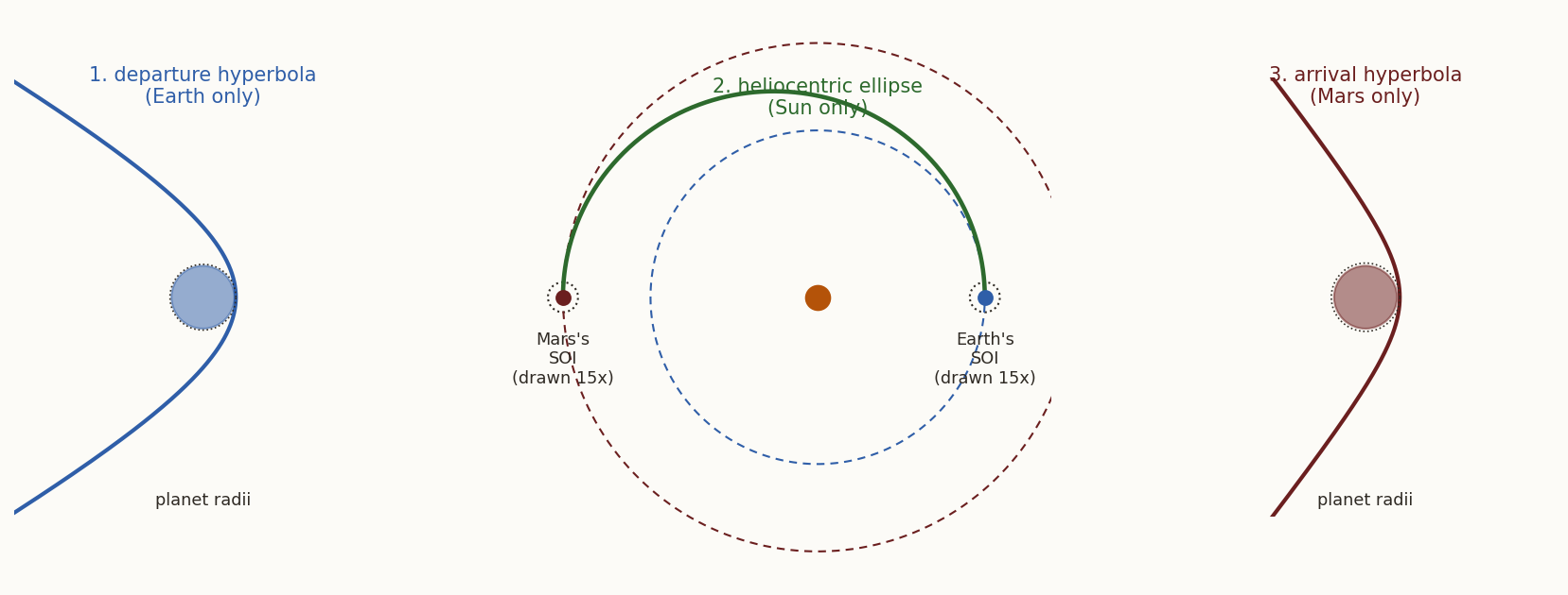
At each boundary the two conics are patched: the spacecraft’s state must be the same on both sides. With the two approximations of the last section, the patch conditions become very simple.
- Position: on the heliocentric conic, the spacecraft is at the planet’s position (the sphere is a point).
- Velocity: the heliocentric velocity and the planet-relative velocity are related by Equation 11, and the planet-relative velocity there is the hyperbola’s \(\mathbf v_\infty\) (the sphere is at infinity):
\[ \mathbf v_\infty=\mathbf V_{\rm s/c}-\mathbf V_{\rm planet}. \tag{19}\]
The excess-speed vector is the whole interface between the heliocentric and the planetary problems. The heliocentric design produces \(\mathbf v_\infty\) at each end; each planetary design takes it as given.
5.2 The algorithm
- Heliocentric transfer. Choose the transfer (for example Hohmann). Find the spacecraft’s heliocentric velocity at departure and at arrival, \(\mathbf V_1\) and \(\mathbf V_2\).
- Excess velocities. \(\mathbf v_{\infty,1}=\mathbf V_1-\mathbf V_{\rm planet\,1}\) and \(\mathbf v_{\infty,2}=\mathbf V_2-\mathbf V_{\rm planet\,2}\).
- Departure. With \(v_{\infty,1}\) and the parking-orbit radius, Equation 9 gives the burn and Equation 6 gives where to make it.
- Arrival. With \(v_{\infty,2}\) and the chosen periapsis, Equation 5 gives the periapsis speed. Then either capture (a burn) or fly by (no burn; Equation 7 gives the turn).
- Timing. The phase angle (Equation 12) gives the launch date; the synodic period gives the next opportunity.
5.3 Where to burn on departure
The burn is at the periapsis of the departure hyperbola. The outgoing asymptote, along which the spacecraft leaves, is at true anomaly \(f_\infty\) from the periapsis. So the burn point is \(f_\infty\) behind the direction in which we want to leave, measured round the parking orbit in the direction of motion. Since \(f_\infty\) lies between \(90^\circ\) and \(180^\circ\), the burn is always made on the far side of the planet from the departure direction.
5.4 Flybys
At a flyby there is no burn. Relative to the planet, the energy \(v_\infty^2/2\) is unchanged, so \(|\mathbf v_\infty^+|=|\mathbf v_\infty^-|\); only the direction turns, through \(\delta\). Relative to the Sun, however,
\[ \mathbf V^\pm=\mathbf V_{\rm planet}+\mathbf v_\infty^\pm , \]
and since \(\mathbf v_\infty\) has turned, \(\mathbf V^+\) need not have the same length as \(\mathbf V^-\). The change in the spacecraft’s heliocentric energy is
\[ \Delta\Bigl(\frac{V^2}{2}\Bigr)=\frac12\Bigl(|\mathbf V_P+\mathbf v_\infty^+|^2-|\mathbf V_P+\mathbf v_\infty^-|^2\Bigr) =\mathbf V_P\cdot\bigl(\mathbf v_\infty^+-\mathbf v_\infty^-\bigr), \tag{20}\]
because \(|\mathbf v_\infty^+|=|\mathbf v_\infty^-|\) and the \(V_P^2\) terms cancel. The heliocentric potential does not change during the flyby (the position is the planet’s, before and after), so this is the whole energy change. The spacecraft gains energy when the turn moves its relative velocity towards the planet’s motion. The energy comes from the planet, whose orbit changes by an unmeasurably small amount.
History. Walter Hohmann published the minimum-energy transfer in Die Erreichbarkeit der Himmelskörper (1925). The gravity assist was worked out in detail by Michael Minovitch at JPL in 1961. The first spacecraft to use one planet to reach another was Mariner 10, which flew past Venus in February 1974 on its way to Mercury.
6 Examples in a plane
In these three examples every orbit lies in one plane: the planets’ orbits are taken as circular and coplanar, and the parking orbits lie in the same plane. The numbers use \(\mu_\odot=1.327\,124\times10^{11}\ \mathrm{km^3/s^2}\), \(1\ \mathrm{AU}=1.495\,979\times10^8\) km, and the planetary data quoted in each example.
6.1 Example 1: from the Earth to Mars
Given. A spacecraft in a \(300\) km circular orbit about the Earth (\(\mu_\oplus=398\,600.4\ \mathrm{km^3/s^2}\), \(R_\oplus=6378.1\) km) is to reach Mars (\(1.52368\) AU, sidereal period \(686.98\) d, \(\mu=42\,828.4\ \mathrm{km^3/s^2}\), \(R=3396.2\) km) on a Hohmann transfer, and be captured there.
Find. (a) The excess speeds at departure and at arrival, and the flight time. (b) The departure burn, and where to make it. (c) How long the spacecraft stays inside the Earth’s sphere of influence. (d) The capture burn into a \(300\) km circular orbit, and into a \(300\times33\,000\) km ellipse; the aim radius. (e) The phase angle at departure, and how often the opportunity recurs.
| symbol | orbit |
|---|---|
| \(V_\oplus\), \(V_{\rm M}\) | circular heliocentric speeds of the Earth and Mars |
| \(V_{t1}\), \(V_{t2}\) | speeds on the heliocentric transfer ellipse, at the Earth and at Mars |
| \(v_{\infty1}\), \(v_{\infty2}\) | excess speeds relative to the Earth and to Mars |
| \(v_c\), \(v_{p1}\) | parking-orbit speed, and periapsis speed of the departure hyperbola |
| \(e_1\), \(e_2\) | eccentricities of the departure and arrival hyperbolas |
Step 1: the heliocentric transfer. With \(r_1=1\) AU, \(r_2=1.52368\) AU and \(a_t=1.26184\) AU, Equation 10 gives
\[ V_\oplus=\sqrt{\mu_\odot/r_1}=29.785\ \mathrm{km/s},\qquad V_{t1}=32.729\ \mathrm{km/s},\qquad V_{\rm M}=24.129\ \mathrm{km/s},\qquad V_{t2}=21.480\ \mathrm{km/s}, \]
and \(t_{12}=\pi\sqrt{a_t^3/\mu_\odot}=258.9\) days.
Step 2: the excess speeds. At departure the transfer velocity and the Earth’s velocity are parallel (both tangential, at perihelion), so \(\mathbf v_{\infty1}\) is along the Earth’s motion with
\[ v_{\infty1}=V_{t1}-V_\oplus=2.945\ \mathrm{km/s}. \]
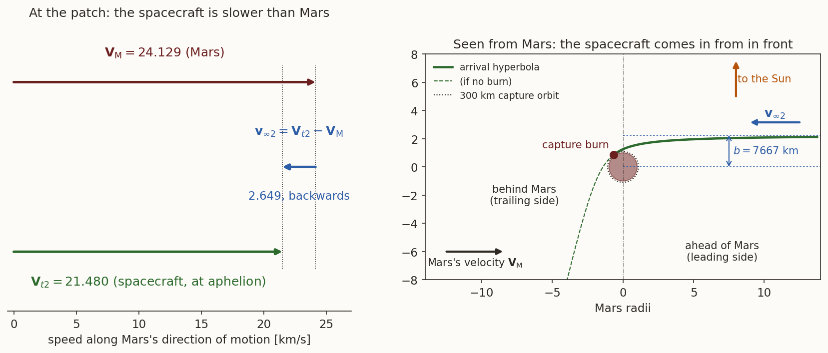
At arrival the spacecraft is at the aphelion of the transfer ellipse, and Mars is at the same point of its circular orbit. Both velocities are again tangential, so they are again parallel, and the excess velocity, Equation 19, is a subtraction along a single line (Figure 4, left):
\[ \mathbf v_{\infty2}=\mathbf V_{t2}-\mathbf V_{\rm M},\qquad v_{\infty2}=|\mathbf V_{t2}-\mathbf V_{\rm M}|=V_{\rm M}-V_{t2}=24.129-21.480=2.649\ \mathrm{km/s}. \]
The order of the two speeds is not an accident of the numbers. Put \(a_t=(r_1+r_2)/2\) in Equation 10:
\[ V_{t2}=\sqrt{\mu_\odot\Bigl(\frac2{r_2}-\frac2{r_1+r_2}\Bigr)}=\sqrt{\frac{\mu_\odot}{r_2}}\sqrt{\frac{2r_1}{r_1+r_2}} =V_{\rm M}\sqrt{\frac{2r_1}{r_1+r_2}}, \]
and the last square root is less than \(1\) because \(r_1<r_2\): the aphelion of a transfer outward is the slowest point of the ellipse, slower than a circular orbit at the same radius. So \(\mathbf v_{\infty2}\) points backwards, opposite to Mars’s motion. At departure it was the other way round: the spacecraft at perihelion was faster than the Earth, and \(\mathbf v_{\infty1}\) pointed forwards.
Why “from in front”. In the Sun’s frame, at the moment of arrival, Mars and the spacecraft move in the same direction along the same line, and Mars is faster by \(2.649\) km/s. Mars is catching up with the spacecraft from behind, as a fast car catches up with a slower one on a road. Now ride on Mars. The spacecraft moves backwards, at \(\mathbf v_{\infty2}\). Something that moves backwards relative to Mars and ends up at Mars must have started ahead of it. The spacecraft therefore enters Mars’s sphere of influence on its leading side, the half that faces the direction in which Mars is moving, and its incoming asymptote runs backwards from there (Figure 4, right). This is the frame in which the arrival hyperbola is drawn, and the aim radius \(b\) of Step 5 is measured from Mars’s centre to that incoming asymptote.
Step 3: the departure burn. At \(r_p=6678.1\) km, the parking orbit has \(v_c=\sqrt{\mu_\oplus/r_p}=7.726\) km/s. The hyperbola’s periapsis speed, Equation 5, is
\[ v_{p1}=\sqrt{2.945^2+\frac{2(398\,600)}{6678.1}}=\sqrt{8.67+119.37}=11.316\ \mathrm{km/s}, \]
so the burn is \(\Delta v_1=11.316-7.726=3.590\) km/s.
Where. \(e_1=1+r_pv_{\infty1}^2/\mu_\oplus=1.1453\), so \(f_\infty=\arccos(-1/1.1453)=150.8^\circ\). The burn is made \(150.8^\circ\) before the point of the parking orbit whose velocity is along the Earth’s heliocentric velocity: on the night side, a little past local midnight (Figure 5).
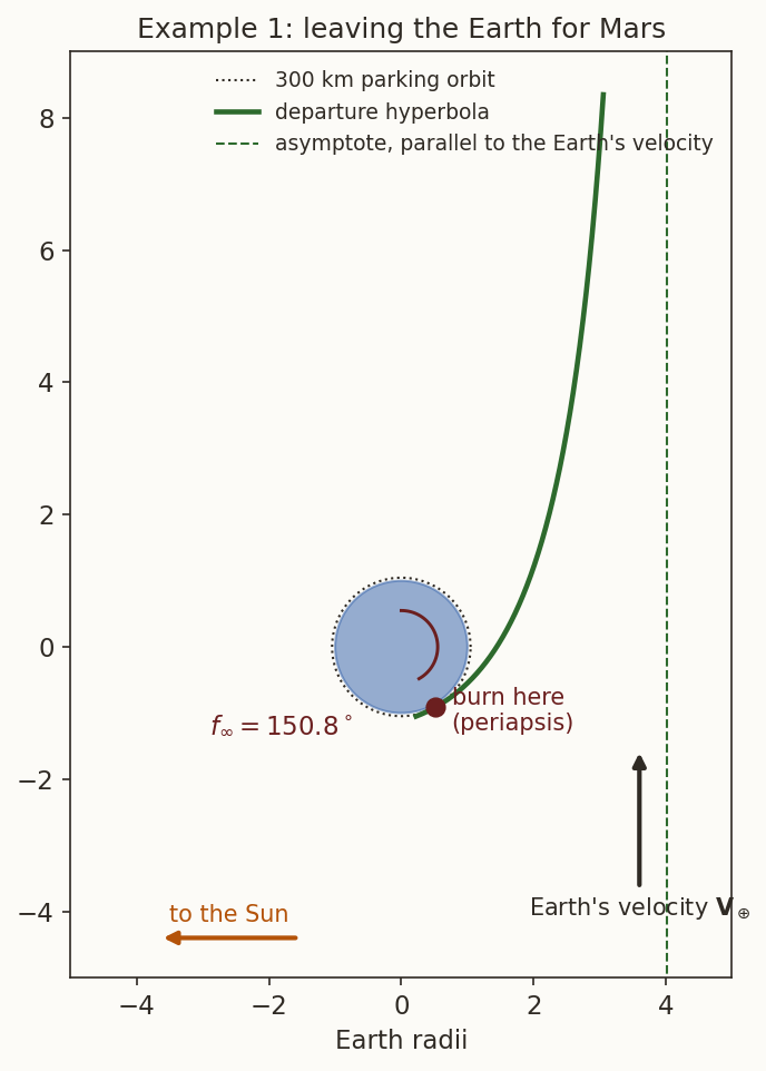
Step 4: time inside the Earth’s sphere of influence. The hyperbola has \(|a|=\mu_\oplus/v_{\infty1}^2=45\,960\) km. On a hyperbola, \(r=|a|(e\cosh F-1)\) and the time from periapsis is \(t=\sqrt{|a|^3/\mu}\,(e\sinh F-F)\), with \(F\) the hyperbolic anomaly. At \(r=r_{\rm SOI}=925\,000\) km, \(\cosh F=(1+r/|a|)/e\) gives \(F=3.61\), and then \(t=3.2\) days. The spacecraft spends \(3\) days of a \(259\)-day trip inside the Earth’s sphere of influence: about \(1\%\) of the time, and \(0.6\%\) of the distance. And there its speed is \(\sqrt{v_{\infty1}^2+2\mu_\oplus/r_{\rm SOI}}=3.088\) km/s, already within \(5\%\) of \(v_{\infty1}\).
Step 5: capture at Mars. At \(r_p=3396.2+300=3696.2\) km the arrival hyperbola has \(v_{p2}=\sqrt{2.649^2+2(42\,828)/3696.2}=5.495\) km/s.
- Into the \(300\) km circle (\(3.404\) km/s): \(\Delta v=2.091\) km/s.
- Into a \(300\times33\,000\) km ellipse (periapsis speed \(4.587\) km/s, period \(23.9\) h): \(\Delta v=0.908\) km/s.
The elliptical capture costs less than half as much, for the reason of Problem 4 of the Indian missions set: only a little speed has to be removed at a periapsis reached at high speed. The spacecraft must be aimed at \(b=r_p\sqrt{1+2\mu/(r_pv_{\infty2}^2)}=7667\) km from Mars’s centre, more than twice the periapsis radius.
Step 6: timing. Mars moves at \(n_{\rm M}=360^\circ/686.98\ \mathrm d\), so in \(258.9\) days it moves \(135.7^\circ\). At launch it must lead the Earth by \(\phi_0=180^\circ-135.7^\circ=44.3^\circ\). The geometry repeats every \(S=1/(1/365.256-1/686.98)=780\) days, about \(2.1\) years.
What the numbers say. The whole interplanetary problem was reduced to two numbers, \(v_{\infty1}\) and \(v_{\infty2}\), and everything else followed from two-body formulas. The Earth’s part of the trip is short and the burn is big; the heliocentric part is long and costs nothing.
6.2 Example 2: to the Moon
The Moon is the hardest case for the method, because its sphere of influence is not small compared with its distance (Section 4). The patch can no longer be at “the Moon’s position”; it must be at a definite point on the Moon’s sphere of influence. This example shows how that is done, and how far the answer is from the truth.
Given. A spacecraft is injected at perigee of a geocentric ellipse, at \(r_0=6678.1\) km (\(300\) km altitude), with speed \(v_0=10.84\) km/s and zero flight-path angle. It is to cross the Moon’s sphere of influence at the point where the line from the Moon makes an angle \(\lambda_1=60^\circ\) with the Moon–Earth line, on the side that the Moon is moving away from. The Moon is on a circle of radius \(D=384\,400\) km, \(\mu_{\rm M}=4902.8\ \mathrm{km^3/s^2}\), \(R_{\rm M}=1737.4\) km.
Find. The geocentric state at the patch, the velocity relative to the Moon there, the perilune, the flight time, and where the Moon must be at injection.
| symbol | orbit |
|---|---|
| \(\varepsilon_0\), \(h_0\), \(e_0\), \(a_0\) | geocentric transfer ellipse |
| \(r_1\), \(v_1\), \(\phi_1\), \(f_1\), \(\gamma_1\) | geocentric state at the patch, and the angle at the Earth between the Moon and the patch |
| \(v_{\rm M}\) | the Moon’s orbital speed |
| \(\mathbf v_2\), \(\varepsilon_2\), \(h_2\), \(e_2\) | selenocentric hyperbola |
Step 1: the Moon’s sphere of influence and speed. \(r_{\rm SOI}=D(\mu_{\rm M}/\mu_\oplus)^{2/5}=66\,183\) km, and \(v_{\rm M}=\sqrt{(\mu_\oplus+\mu_{\rm M})/D}=1.0245\) km/s.
Step 2: the geocentric ellipse. \(\varepsilon_0=v_0^2/2-\mu_\oplus/r_0=-0.9346\ \mathrm{km^2/s^2}\), so \(a_0=-\mu_\oplus/2\varepsilon_0=213\,253\) km; \(h_0=r_0v_0=72\,391\ \mathrm{km^2/s}\), \(p_0=h_0^2/\mu_\oplus=13\,147\) km and \(e_0=p_0/r_0-1=0.9687\). Its apogee would be at \(419\,828\) km, beyond the Moon.
Step 3: the patch point. In the triangle Earth–Moon–patch point, two sides (\(D\) and \(r_{\rm SOI}\)) and the angle between them (\(\lambda_1\)) are known. The cosine rule gives the distance from the Earth,
\[ r_1=\sqrt{D^2+r_{\rm SOI}^2-2Dr_{\rm SOI}\cos\lambda_1}=355\,953\ \mathrm{km}, \]
and the sine rule the angle at the Earth between the Moon and the patch point, \(\sin\gamma_1=(r_{\rm SOI}/r_1)\sin\lambda_1\), so \(\gamma_1=9.27^\circ\).
Step 4: the geocentric state at the patch. Energy and angular momentum are conserved on the ellipse:
\[ v_1=\sqrt{2\Bigl(\varepsilon_0+\frac{\mu_\oplus}{r_1}\Bigr)}=0.6087\ \mathrm{km/s},\qquad \cos\phi_1=\frac{h_0}{r_1v_1}\ \Rightarrow\ \phi_1=70.48^\circ . \]
The flight-path angle is large: the spacecraft is still climbing steeply when it reaches the Moon’s neighbourhood. Its true anomaly there is \(f_1=\arccos\bigl((p_0/r_1-1)/e_0\bigr)=173.83^\circ\), and Kepler’s equation (\(E_1=2.3334\) rad) gives the flight time from injection, \(t_1=70.75\) h.
Step 5: the velocity relative to the Moon. This is the patch: Equation 19, with the Moon as the planet. The Moon’s velocity is perpendicular to the Earth–Moon line; the spacecraft’s is at \(\phi_1\) from the perpendicular to its own radius, which is turned by \(\gamma_1\) from the Moon’s. So the angle between the two velocity vectors is \(\phi_1-\gamma_1=61.21^\circ\), and
\[ v_2=\sqrt{v_1^2+v_{\rm M}^2-2v_1v_{\rm M}\cos(\phi_1-\gamma_1)}=0.9053\ \mathrm{km/s}. \]
Step 6: the selenocentric hyperbola. At the patch point the spacecraft is \(r_{\rm SOI}\) from the Moon with speed \(v_2\):
\[ \varepsilon_2=\frac{v_2^2}{2}-\frac{\mu_{\rm M}}{r_{\rm SOI}}=0.3357\ \mathrm{km^2/s^2}>0, \qquad v_\infty=\sqrt{2\varepsilon_2}=0.819\ \mathrm{km/s}. \]
The selenocentric orbit is a hyperbola: without a burn the spacecraft cannot stay. Its angular momentum is \(h_2=|\boldsymbol\rho\times\mathbf v_2|=6371\ \mathrm{km^2/s}\), with \(\boldsymbol\rho\) the vector from the Moon to the patch point. (It is negative about the Earth’s orbit normal: the spacecraft goes round the Moon the opposite way to the Moon’s motion round the Earth.) Then \(e_2=\sqrt{1+2\varepsilon_2h_2^2/\mu_{\rm M}^2}=1.4607\) and
\[ r_{p}=\frac{h_2^2/\mu_{\rm M}}{1+e_2}=3364\ \mathrm{km}, \]
a perilune altitude of \(1627\) km. On the hyperbola (\(|a_2|=\mu_{\rm M}/v_\infty^2=7302\) km) the time from the patch to perilune is \(18.2\) h, so the whole flight takes \(88.9\) h.
Step 7: where the Moon must be at injection. In \(t_1=70.75\) h the Moon moves through \(n_{\rm M}t_1=38.9^\circ\). At the patch it is at geocentric angle \(f_1-\gamma_1=164.56^\circ\) from the injection point, so at injection it must be \(164.56^\circ-38.90^\circ=125.66^\circ\) ahead of it.
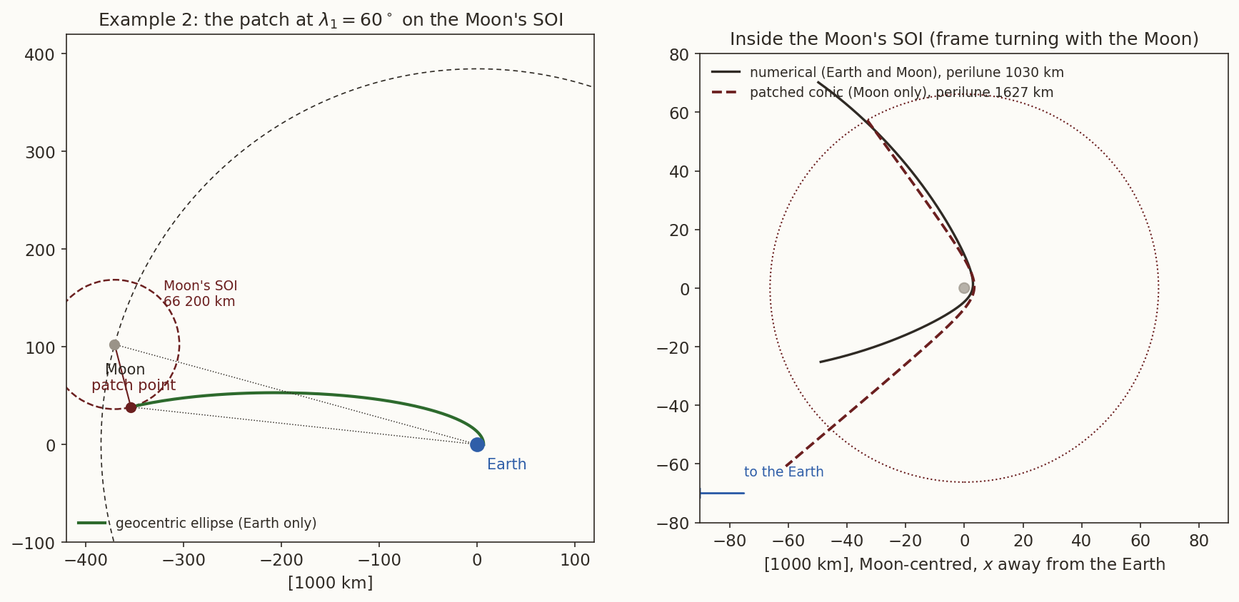
Step 8: how sensitive is it? Repeating Steps 3 to 6 for nearby \(\lambda_1\) shows that the perilune altitude changes by about \(600\) km per degree of \(\lambda_1\). A perilune of \(200\) km needs \(\lambda_1=57.49^\circ\). A lunar trajectory is extremely sensitive to the injection conditions, which is why every lunar mission flies trajectory-correction burns.
Step 9: the truth. Integrating the same injection numerically, with the Earth and the Moon both pulling throughout (Figure 6), gives a perilune altitude of about \(1030\) km at \(87.0\) h. The patched conic is \(600\) km off in perilune and \(2\) hours off in time. For the Moon, the patched conic is a good first guess to start a numerical search, not an answer.
6.3 Example 3: a flyby of Jupiter
Given. A spacecraft reaches Jupiter (\(5.2026\) AU, \(\mu_J=1.266\,865\times10^8\ \mathrm{km^3/s^2}\), \(R_J=71\,492\) km) at the aphelion of a Hohmann transfer from the Earth. It flies past Jupiter with periapsis \(r_p=5R_J\), passing behind Jupiter (on the side Jupiter is moving away from).
Find. The turning angle, the heliocentric velocity after the flyby, the energy gained, and the new heliocentric orbit. Can any flyby of this kind send the spacecraft out of the solar system?
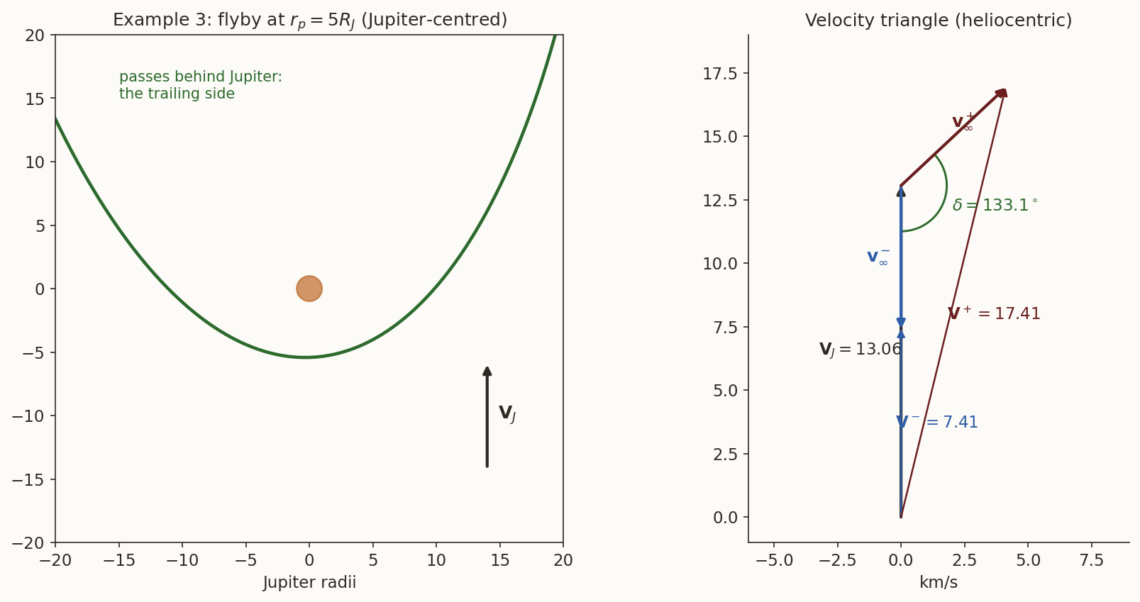
Step 1: arrival. \(a_t=(1+5.2026)/2\) AU; at aphelion \(V^-=V_{t2}=7.415\) km/s, while Jupiter moves at \(V_J=13.058\) km/s. The spacecraft is overtaken by Jupiter, and relative to Jupiter it moves backwards with \(v_\infty=V_J-V^-=5.643\) km/s. The trip took \(2.73\) years.
Step 2: the turn. \(e=1+r_pv_\infty^2/\mu_J=1+\dfrac{357\,460\times31.85}{1.2669\times10^8}=1.0899\), so \(\delta=2\arcsin(1/e)=133.1^\circ\).
Step 3: the velocity triangle. Take Jupiter’s velocity along \(+y\), so \(\mathbf v_\infty^-=(0,-5.643)\) km/s. Passing behind Jupiter turns \(\mathbf v_\infty\) by \(133.1^\circ\) towards \(+x\):
\[ \mathbf v_\infty^+=v_\infty(\sin\delta,\ -\cos\delta)=(4.118,\ 3.859)\ \mathrm{km/s},\qquad \mathbf V^+=\mathbf V_J+\mathbf v_\infty^+=(4.118,\ 16.917)\ \mathrm{km/s}. \]
The heliocentric speed has gone from \(7.41\) to \(|\mathbf V^+|=17.41\) km/s (Figure 7). The relative speed is \(5.643\) km/s before and after; only its direction changed.
Step 4: the energy. By Equation 20, \(\Delta(V^2/2)=\mathbf V_J\cdot(\mathbf v_\infty^+-\mathbf v_\infty^-)=13.058\times(3.859+5.643)=124.1\ \mathrm{km^2/s^2}\). The new heliocentric energy is \(V^{+2}/2-\mu_\odot/r=-18.95\ \mathrm{km^2/s^2}\), still negative: the spacecraft is still bound to the Sun. Its new orbit has \(a=23.4\) AU and \(e=0.79\): perihelion \(4.87\) AU, aphelion \(42\) AU, beyond Neptune.
Step 5: can it escape? Solar escape speed at Jupiter’s distance is \(\sqrt{2\mu_\odot/r}=18.47\) km/s. With \(|\mathbf V^+|^2=V_J^2+v_\infty^2-2V_Jv_\infty\cos\delta\), reaching it needs \(\cos\delta=-0.941\), \(\delta=160.2^\circ\), and so \(e=1/\sin(80.1^\circ)=1.0151\) and \(r_p=(e-1)\mu_J/v_\infty^2=60\,100\) km. That is inside Jupiter (\(R_J=71\,492\) km). Even a grazing flyby (\(r_p=R_J\)) turns the velocity by only \(158.4^\circ\) and gives \(18.42\) km/s, just short. A Hohmann arrival at Jupiter is too slow to be flung out of the solar system; the probes that left the solar system after a Jupiter flyby, starting with Pioneer 10 in 1973, arrived faster than Hohmann (Pioneer 10 took 21 months, against the Hohmann transfer’s \(2.7\) years).
What the numbers say. No propellant was spent, yet the heliocentric speed more than doubled. The rule of Equation 20 explains the side: passing behind the planet turns \(\mathbf v_\infty\) towards the planet’s own motion, and \(\mathbf V_J\cdot\Delta\mathbf v_\infty>0\).
7 Examples out of the plane
7.1 What changes in three dimensions
In three dimensions \(\mathbf v_\infty\) is a direction in space, not just a speed, and that direction need not lie in any convenient plane. Two new questions arise.
Which planetary orbits contain a given asymptote? Every hyperbola leaving along a direction \(\hat{\mathbf s}\) lies in a plane that contains \(\hat{\mathbf s}\). There is a whole family of such planes, obtained by turning one of them about \(\hat{\mathbf s}\). Let \(\delta_\infty\) be the declination of \(\hat{\mathbf s}\) above the planet’s equator. To find the inclinations of the planes of the family, build two unit vectors perpendicular to \(\hat{\mathbf s}\):
\[ \hat{\mathbf e}_1=\frac{\hat{\mathbf K}\times\hat{\mathbf s}}{|\hat{\mathbf K}\times\hat{\mathbf s}|},\qquad \hat{\mathbf e}_2=\hat{\mathbf s}\times\hat{\mathbf e}_1 , \]
with \(\hat{\mathbf K}\) the planet’s pole. Since \(|\hat{\mathbf K}\times\hat{\mathbf s}|=\cos\delta_\infty\), \(\hat{\mathbf K}\cdot\hat{\mathbf e}_1=0\) and \(\hat{\mathbf K}\cdot\hat{\mathbf e}_2=\hat{\mathbf e}_1\cdot(\hat{\mathbf K}\times\hat{\mathbf s})=\cos\delta_\infty\). Any orbit normal of the family is \(\hat{\mathbf h}=\cos\theta\,\hat{\mathbf e}_1+\sin\theta\,\hat{\mathbf e}_2\), and its inclination is
\[ \cos i=\hat{\mathbf h}\cdot\hat{\mathbf K}=\cos\delta_\infty\,\sin\theta . \tag{21}\]
As \(\theta\) varies, \(\cos i\) ranges between \(\pm\cos\delta_\infty\):
\[ |\delta_\infty|\ \le\ i\ \le\ 180^\circ-|\delta_\infty| . \tag{22}\]
An orbit plane can only contain an asymptote whose declination is no larger than its inclination. This is the same relation that ties a launch site’s latitude to the smallest inclination it can reach directly (the Orbital Elements deck): there the direction is the radius to the launch site, here it is the asymptote.
How does the heliocentric transfer reach a target out of the ecliptic? The heliocentric conic must lie in a plane through the Sun, the departure point and the arrival point. If those three are nearly in a line (a transfer of nearly \(180^\circ\)) the plane is badly determined, and a target slightly out of the ecliptic forces a steeply inclined transfer. Example 5 shows how expensive that is, and the usual remedy.
7.2 Example 4: the departure asymptote and the launch site
Given. The Hohmann departure of Example 1, \(v_{\infty1}=2.945\) km/s, with \(\mathbf v_{\infty1}\) along the Earth’s heliocentric velocity (in the ecliptic). The Earth’s equator is inclined to the ecliptic by \(\varepsilon=23.44^\circ\). The parking orbit is reached by launching from Sriharikota, latitude \(13.72^\circ\) N.
Find. (a) The declination \(\delta_\infty\) of the departure asymptote, relative to the Earth’s equator, as a function of the date. (b) Its value for a departure on about 30 November (\(\lambda_\odot=248^\circ\)) and on about 20 March (\(\lambda_\odot=0^\circ\)). (c) Whether a parking orbit launched due east from Sriharikota can contain the asymptote; if not, the launch azimuth that can, or the cost of a combined plane change.
Step 1: where the Earth’s velocity points. On the day when the Sun’s ecliptic longitude is \(\lambda_\odot\), the Earth is at heliocentric longitude \(\lambda_\odot+180^\circ\), and its velocity is \(90^\circ\) ahead of that, at ecliptic longitude \(\lambda_v=\lambda_\odot+270^\circ=\lambda_\odot-90^\circ\) and ecliptic latitude \(0\).
Step 2: its declination. A direction in the ecliptic at longitude \(\lambda_v\) has declination \(\sin\delta=\sin\varepsilon\sin\lambda_v\) (the ecliptic is the equator tilted by \(\varepsilon\) about the equinox line). So
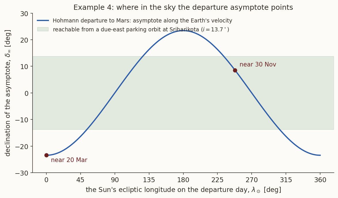
\[ \sin\delta_\infty=\sin\varepsilon\,\sin(\lambda_\odot-90^\circ)=-\sin\varepsilon\cos\lambda_\odot . \]
Figure 8 plots it over the year. It swings between \(\pm23.44^\circ\): in March the asymptote points far south, in September far north, and near the solstices it lies in the equator.
Step 3: the two dates.
- 30 November, \(\lambda_\odot=248^\circ\): \(\sin\delta_\infty=-0.3978\cos248^\circ=0.149\), so \(\delta_\infty=8.57^\circ\).
- 20 March, \(\lambda_\odot=0^\circ\): \(\delta_\infty=-23.44^\circ\).
Step 4: can the parking orbit contain the asymptote? By Equation 22, the parking orbit needs \(i\ge|\delta_\infty|\). A due-east launch from Sriharikota gives \(i=13.72^\circ\).
- In November, \(8.57^\circ<13.72^\circ\): yes. The departure plane is the parking orbit’s plane, and the burn of Example 1 is all that is needed.
- In March, \(23.44^\circ>13.72^\circ\): no. Either launch into a more inclined parking orbit, with azimuth \(\beta\) from \(\cos i=\cos\phi\sin\beta\): \(\sin\beta=\cos23.44^\circ/\cos13.72^\circ=0.9444\), so \(\beta=70.8^\circ\) or \(109.2^\circ\) (a little north or south of east); or keep the due-east orbit and turn the velocity out of its plane during the departure burn.
Step 5: the cost of turning during the burn. The smallest tilt that brings the departure plane to the asymptote is \(\alpha=23.44^\circ-13.72^\circ=9.72^\circ\). A burn that takes the speed from \(v_c=7.726\) to \(v_{p1}=11.316\) km/s and turns the velocity through \(\alpha\) costs, by the cosine rule,
\[ \Delta v=\sqrt{v_c^2+v_{p1}^2-2v_cv_{p1}\cos\alpha}=3.924\ \mathrm{km/s}, \]
\(334\) m/s more than the coplanar \(3.590\) km/s. A \(9\%\) larger departure burn may or may not be cheaper than a less efficient launch azimuth; the trade is a launch-vehicle question.
What the numbers say. The heliocentric problem fixes \(\mathbf v_\infty\) as a vector. Its direction, seen from the Earth, depends on the date, and the parking orbit must be chosen to contain it. Launch sites near the equator can reach a wider band of declinations without paying.
7.3 Example 5: a target out of the ecliptic
Given. The Earth–Mars Hohmann transfer of Example 1, but now Mars’s orbit is inclined to the ecliptic by \(1.85^\circ\), and on the arrival date Mars is at its greatest ecliptic latitude, \(\beta=1.85^\circ\). The Earth’s orbit is the ecliptic.
Find. (a) Why a transfer of exactly \(180^\circ\) cannot reach Mars. (b) The cost of tilting the whole transfer so that a transfer of slightly less than \(180^\circ\) reaches Mars. (c) The cost of a broken-plane transfer instead.
Step 1: the \(180^\circ\) problem. The transfer plane must contain the Sun, the Earth’s position at departure and Mars’s position at arrival. In a Hohmann transfer those three are in a line, and the plane through a line and a point on that line is undetermined. If Mars is slightly off the line (above the ecliptic), the only plane through all three is the one containing the line and the small offset, and that plane is nearly perpendicular to the ecliptic. Flying it would mean leaving the Earth almost at right angles to its orbit: hopeless.
Step 2: tilting the transfer. Shorten the transfer to an angle \(\Theta<180^\circ\), with its line of nodes through the departure point. A point \(\Theta\) round an orbit inclined at \(i_t\) from its node has latitude given by \(\sin\beta=\sin i_t\sin\Theta\) (the Orbital Elements relation \(\sin\delta=\sin i\sin u\)). So
\[ \sin i_t=\frac{\sin\beta}{\sin\Theta}. \]
To keep the arithmetic simple, keep the Hohmann speeds and only tilt the departure velocity. The spacecraft must leave at \(V_{t1}=32.729\) km/s, inclined at \(i_t\) to the Earth’s \(V_\oplus=29.785\) km/s, and by the cosine rule
\[ v_{\infty1}=\sqrt{V_{t1}^2+V_\oplus^2-2V_{t1}V_\oplus\cos i_t}. \]
| \(\Theta\) | \(i_t\) | \(v_{\infty1}\) [km/s] | \(\Delta v\) from \(300\) km [km/s] |
|---|---|---|---|
| \(150^\circ\) | \(3.70^\circ\) | \(3.57\) | \(3.77\) |
| \(160^\circ\) | \(5.42^\circ\) | \(4.17\) | \(3.97\) |
| \(170^\circ\) | \(10.71^\circ\) | \(6.53\) | \(5.00\) |
| \(175^\circ\) | \(21.74^\circ\) | \(12.14\) | \(8.61\) |
Near \(180^\circ\) the cost explodes. Even at \(\Theta=170^\circ\) the departure burn grows by \(1.4\) km/s, because a \(10.7^\circ\) tilt of a \(33\) km/s velocity is a big vector change.
Step 3: the broken-plane transfer. Leave in the ecliptic on the Hohmann ellipse, and change the plane on the way, at a point \(90^\circ\) before arrival. A plane change of \(\Delta i\) made at a point \(90^\circ\) before the target reaches a latitude \(\Delta i\) at the target (again \(\sin\beta=\sin\Delta i\sin90^\circ\)), so \(\Delta i=\beta=1.85^\circ\) suffices. That point is at true anomaly \(90^\circ\) on the transfer ellipse, at \(r=p_t=1.2075\) AU, where the transverse velocity is \(V_\theta=h_t/r=27.10\) km/s. Turning the plane about the radius vector rotates only the transverse component:
\[ \Delta v_{\rm break}=2V_\theta\sin\frac{\Delta i}{2}=0.875\ \mathrm{km/s}. \]
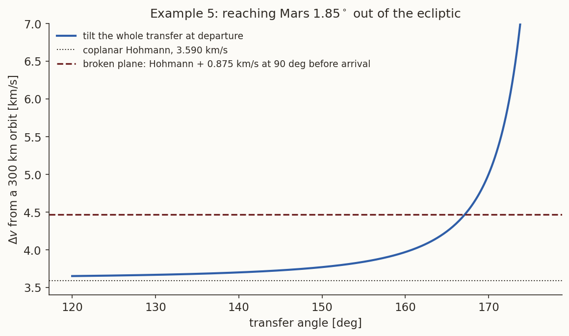
What the numbers say. The broken-plane transfer costs \(3.590+0.875=4.47\) km/s in all. That is better than tilting the transfer at departure whenever \(\Theta\) exceeds about \(167^\circ\) (Figure 9), and it keeps the near-Hohmann geometry. The cheapest option of all is to choose the dates so that Mars is near a node of its orbit on arrival (\(\beta\approx0\)): then no plane change is needed. This is one reason why real transfers are rarely exactly \(180^\circ\) (Problem 4 of the Indian missions set: Mangalyaan’s transfer swept \(218^\circ\)).
7.4 Example 6: arriving at Mars out of its equator
Given. The Mars Orbiter Mission’s arrival, reconstructed in Problem 4 of the Indian missions set: \(v_\infty=3.155\) km/s, along a direction whose declination relative to Mars’s equator is \(\delta_\infty=-30.25^\circ\) (from the Lambert arc between the actual dates and Mars’s pole direction). The capture orbit was \(421.7\times76\,993.6\) km with inclination \(150.0^\circ\) to Mars’s equator.
Find. (a) The inclinations that a capture orbit can have without a plane change. (b) Whether MOM’s orbit is one of them. (c) The cost of an equatorial capture orbit instead: turning the plane during the insertion burn, or later at apoapsis.
Step 1: the family of planes. By Equation 21, \(\cos i=\cos30.25^\circ\sin\theta=0.864\sin\theta\), so \(30.25^\circ\le i\le149.75^\circ\) (Figure 10). Which member is flown is chosen by aiming: the angle \(\theta\) is the direction of the miss vector around the asymptote, in the plane perpendicular to it (the “B-plane”), and is set by the trajectory corrections on the way in.
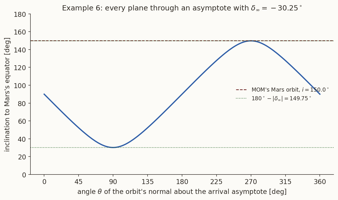
Step 2: MOM’s orbit. \(150.0^\circ\) lies at the upper edge of the range, within the accuracy of the reconstruction: MOM’s orbit is the most nearly equatorial (retrograde) orbit that this arrival direction allows without a plane change. That edge is reached when \(\sin\theta=-1\), i.e. when the orbit normal is as close as possible to Mars’s south pole.
Step 3: an equatorial orbit instead. Reaching \(i=180^\circ\) needs a further plane change of \(30.25^\circ\). Two places to do it:
- During the insertion burn, at periapsis. The burn must take the hyperbola’s \(5.691\) km/s to the orbit’s \(4.628\) km/s and turn it through \(30.25^\circ\): \(\sqrt{5.691^2+4.628^2-2(5.691)(4.628)\cos30.25^\circ}=2.881\) km/s, against \(1.063\) km/s coplanar.
- Later, at apoapsis, where the capture orbit moves at only \(0.220\) km/s: \(2(0.220)\sin15.125^\circ=0.115\) km/s.
What the numbers say. The arrival direction limits the capture inclinations exactly as the launch site’s latitude limits the parking orbit’s. When a different plane is wanted, a high-apoapsis capture orbit lets the plane change be made where the spacecraft is slow: \(0.115\) km/s instead of \(1.8\) km/s extra.
8 The method against the truth
The patched-conic method neglects, by construction, an \(8\%\) perturbation at the edge of each sphere of influence (Section 4). Two numerical checks show what that does.
Earth to Mars (Example 1). Integrating the departure from the \(300\) km orbit with both the Sun and the Earth pulling all the time, with the patched-conic burn of \(3.590\) km/s, gives an aphelion of \(1.5271\) AU, not \(1.5237\) AU: about \(510\,000\) km beyond Mars’s orbit. The burn that does reach \(1.5237\) AU in the integration is \(3.586\) km/s. The patched conic overestimates the burn by \(3.8\) m/s (\(0.1\%\)), and that tiny error misses the target by half a million km. The method is excellent for the \(\Delta v\) budget, and inadequate for aiming.
Earth to the Moon (Example 2). The patched conic’s perilune is \(1627\) km; the integration gives \(1030\) km. The Moon’s sphere of influence is not small compared with the Earth–Moon distance, and the Earth keeps pulling hard inside it.
So the patched-conic method is the first step of mission design, not the last. It gives the launch window, the \(\Delta v\) budget, the burn locations and a first guess at the trajectory. That guess is then refined by numerical integration of the full equations, and in flight by trajectory-correction manoeuvres.
9 Summary
- The motion of a spacecraft can be written about the planet or about the Sun; each is a two-body problem plus a perturbation (Equation 14, Equation 15). The Sun’s perturbation of motion about the planet is tidal: the difference between its pulls on spacecraft and planet.
- Laplace’s criterion picks the description with the smaller relative perturbation. The boundary is \(r_{\rm SOI}=R(m/M)^{2/5}\): \(925\,000\) km for the Earth, \(66\,200\) km for the Moon. At the boundary the neglected perturbation is still about \((m/M)^{1/5}\) of the main pull.
- Patched conics: one two-body problem per region. At each patch the position is the planet’s and the velocity obeys \(\mathbf v_\infty=\mathbf V-\mathbf V_{\rm planet}\). The vector \(\mathbf v_\infty\) is the whole interface between the heliocentric and the planetary designs.
- Departure and capture are periapsis burns, \(\Delta v=\sqrt{v_\infty^2+2\mu/r_p}-v_{\rm orbit}\); the departure burn is \(f_\infty=\arccos(-1/e)\) before the asymptote.
- A flyby keeps \(|\mathbf v_\infty|\) and turns it through \(\delta=2\arcsin(1/e)\); the heliocentric energy changes by \(\mathbf V_P\cdot\Delta\mathbf v_\infty\).
- Out of the plane: an orbit can contain an asymptote only if \(i\ge|\delta_\infty|\); near-\(180^\circ\) transfers to inclined targets are ruinous, and a broken-plane transfer or a better choice of dates avoids them.
- The method gives budgets to \(0.1\%\), but aiming errors of \(10^5\) km at a planet and hundreds of km at the Moon: it is the starting point for numerical refinement.
Every number in this note is recomputed by codes/patched-conics-verify.py, including the two numerical integrations of Section 8. The figures are drawn by codes/fig-pc-patched-conics.py.