Orbital Elements
Six numbers that place an orbit in space: the reference frame, the three angles, and the two maps between elements and state vectors
1 Where we are going
The two-body note gave us the orbit in its own plane: a conic
\[ r=\frac{p}{1+e\cos f},\qquad p=\frac{h^2}{\mu}=a(1-e^2), \]
with the attracting body at a focus and the true anomaly \(f\) measured from periapsis. That is enough to say how far away a satellite is and how fast it moves. It is not enough to point an antenna at it, to know which part of the Earth it flies over, or to tell whether two satellites might collide. For that we need to know how the orbital plane, and the conic inside it, sit in space.
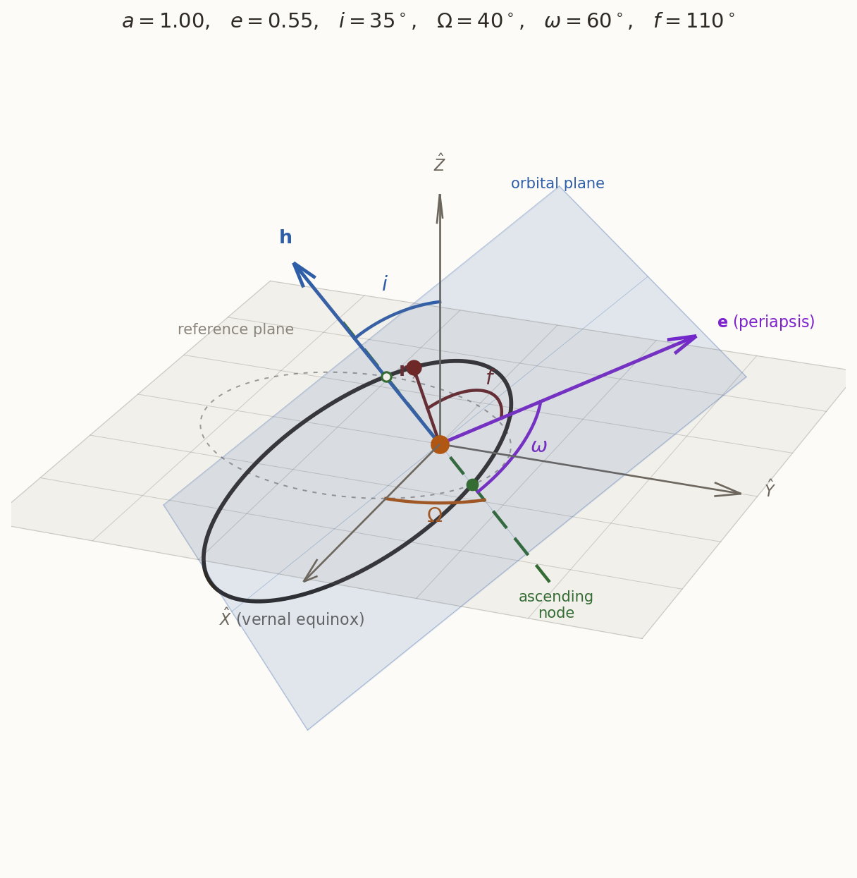
This note answers that question. The orientation turns out to need three angles, so that an orbit is fixed by six numbers, the classical orbital elements (Figure 1): two for the conic (\(a\) and \(e\)), three for its orientation (\(i\), \(\Omega\), \(\omega\)), and one for where the body is on it (\(f\)).
The route:
- Section 2: why exactly six numbers.
- Section 3: angles need a reference frame; we build the standard one for Earth orbits, and see why even it is not perfectly fixed.
- Section 4: we define \(i\), \(\Omega\), \(\omega\), and show that three vectors, \(\mathbf h\), \(\mathbf n\) and \(\mathbf e\), measure them.
- Section 5: from a state vector \((\mathbf r,\mathbf v)\) to the elements, where all but one of the angles comes out in the wrong quadrant half the time unless we are careful.
- Section 6: from the elements back to \((\mathbf r,\mathbf v)\).
- Section 7: five worked examples.
As before, a blue Try it box asks you to do something, and a green Check yourself box asks a short question; each has a hidden answer. Throughout, \(\mu=398\,600\) km\(^3\)/s\(^2\) and \(R_\oplus=6378.137\) km; angles are quoted in degrees and computed in radians.
When you finish, you should be able to answer the following.
- Why does an orbit need exactly six numbers, and why is one of them different from the other five?
- What is the vernal equinox, and why must every orbit be given with an epoch?
- Why is every sun-synchronous orbit retrograde?
- When you compute \(\Omega\), \(\omega\) and \(f\) from a state vector, how do you know which quadrant they are in?
- Why does a quadrant error leave every length correct and still put the satellite on the other side of the Earth?
2 Why exactly six numbers?
The two-body equation \(\ddot{\mathbf r}=-\mu\mathbf r/r^3\) is a second-order vector ODE in three dimensions, i.e. six first-order scalar ODEs. Its general solution therefore carries six constants of integration. The state \((\mathbf r,\mathbf v)\) at one instant is one legitimate choice of the six. The classical elements are another, built from the integrals we already have:
\[ \mathbf h=\mathbf r\times\mathbf v\ \ (3),\qquad \mathbf e=\frac{\mathbf v\times\mathbf h}{\mu}-\hat{\mathbf r}\ \ (3),\qquad t_p\ \ (1). \]
That is seven numbers. Which relation removes one of them?
Answer
\(\mathbf h\cdot\mathbf e=0\): the eccentricity vector lies in the orbital plane. So \(\mathbf h\) and \(\mathbf e\) carry five independent numbers, and the time of periapsis passage \(t_p\) is the sixth.\[ \boxed{\;5\ \text{constants that fix the orbit}\;+\;1\ \text{constant that fixes the clock}\;=\;6 .\;} \]
Five of the six elements describe a curve that does not change; the sixth says where on the curve the body is, and it is the only one that runs with time. Keep this split in mind: it organises everything below.
3 A frame to measure angles in
An angle is measured from something. Before we can orient an orbit we need fixed reference directions, and the honest answer to “fixed with respect to what?” turns out to be surprisingly subtle.
3.1 Directions on the sky
Astronomers describe directions as points on the celestial sphere: a sphere of arbitrary radius centred on the Earth, on which only direction matters. Four terms are needed.
- The celestial equator is the great circle in which the plane of the Earth’s equator cuts the celestial sphere: the terrestrial equator projected onto the sky. Its poles are the celestial poles, directly above the Earth’s poles.
- An hour circle is a great circle through both celestial poles and the object: the sky’s version of a meridian of longitude. The observer’s meridian is the hour circle through the observer’s zenith; a body is at its highest (it culminates) when it crosses it, and for the Sun that moment is apparent noon.
- The declination \(\delta\in[-90^\circ,90^\circ]\) of an object is its angle from the celestial equator, measured along its hour circle, positive north: the sky’s latitude.
- The right ascension \(\alpha\in[0^\circ,360^\circ)\) is the angle, measured eastward along the celestial equator, from a reference direction \(\hat{\mathbf I}\) to the object’s hour circle: the sky’s longitude. It is often quoted in hours, \(24^{\rm h}=360^\circ\).
In a Cartesian frame \(\{\hat{\mathbf I},\hat{\mathbf J},\hat{\mathbf K}\}\) with \(\hat{\mathbf K}\) along the Earth’s axis, these are just spherical coordinates:
\[ \hat{\mathbf r}=\left(\cos\delta\cos\alpha,\ \cos\delta\sin\alpha,\ \sin\delta\right). \]
So \(\delta=0\) means “in the equatorial plane”, and \(\alpha\) is measured from a direction in that plane that we have not yet chosen. How do we choose it? Look at the Sun.
3.2 A year of noons
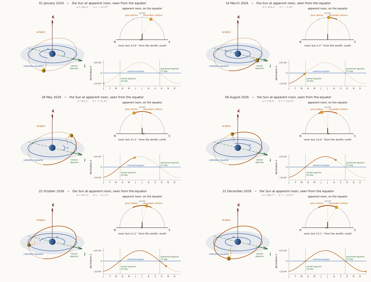
Watch Figure 2. On the equator, at apparent noon, the zenith is on the celestial equator, so the Sun’s distance from the zenith equals its declination \(|\delta|\), and a vertical stick’s noon shadow measures it. (a) Between what limits does \(\delta\) swing over the year? (b) On how many days is there no noon shadow? (c) What would the noon zenith distance be at latitude \(\varphi\)?
What you should find
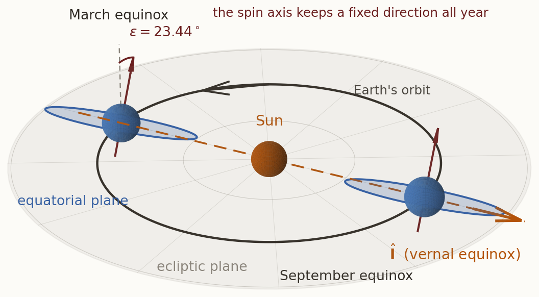
Between \(\pm23.44^\circ\): the Sun is not in the equatorial plane. It moves round the ecliptic, the plane of the Earth’s orbit, which is tilted by the obliquity \(\varepsilon=23.44^\circ\) to the equator.
Two: the days when \(\delta=0\) and the Sun lies in the equatorial plane, the equinoxes (in 2026, 20 March and 23 September).
\(|\varphi-\delta|\).
The two planes, equator and ecliptic, meet in a line, and the Sun lies on that line at the two equinoxes. At the March equinox the Sun crosses the equator going north; this is the vernal equinox, and the direction from the Earth to the Sun at that moment is the reference direction \(\hat{\mathbf I}\) (Figure 3). Right ascension is measured from it.
3.3 The geocentric equatorial frame
The standard frame for Earth orbits, often called ECI (Earth-centred inertial), is:
- origin at the centre of the Earth;
- \(\hat{\mathbf I}\) towards the vernal equinox \(\Upsilon\);
- \(\hat{\mathbf K}\) along the Earth’s rotation axis, towards the north pole;
- \(\hat{\mathbf J}=\hat{\mathbf K}\times\hat{\mathbf I}\), completing a right-handed set.
The \(\hat{\mathbf I}\hat{\mathbf J}\) plane, the equator, is the reference plane. (For orbits about the Sun the reference plane is the ecliptic instead; every definition below is unchanged.)
3.4 The axes do not hold still
The frame is built from two planes, the equator and the ecliptic. If either moves, so do the axes. Both move.
The Earth’s axis precesses. The Earth is slightly flattened, and the Sun and Moon pull harder on the near side of its equatorial bulge than on the far side. The resulting torque tries to tip the equator into the ecliptic; a spinning body answers a torque at right angles to it, so the axis instead sweeps out a cone of half-angle \(\varepsilon\), at about \(50.3''\) per year: one turn in about \(25\,770\) years (the Moon supplies about two thirds of the effect, the Sun one third). On top of the cone the axis nods (nutation), mainly with the \(18.6\)-year period of the Moon’s orbital node, by \(9.2''\) in obliquity and \(17.2''\) in longitude. Meanwhile the planets slowly tilt the ecliptic itself, by about \(47''\) per century, which makes the obliquity drift (it oscillates between about \(22.1^\circ\) and \(24.5^\circ\) over some \(41\,000\) years).
So \(\hat{\mathbf I}\), the intersection of two moving planes, slides westward along the ecliptic, about \(1^\circ\) every \(72\) years.
The vernal equinox is called the “First Point of Aries”. At \(1^\circ\) per \(72\) years, how long does it take to cross one \(30^\circ\) sign of the zodiac? Is it still in Aries?
Answer
About \(2150\) years. It was in Aries when it was named, about two thousand years ago; it crossed into Pisces around 68 BC, is there now, and will reach Aquarius around 2600 AD. The name is a fossil.History: Hipparchus and precession. Hipparchus discovered precession around 130 BC by comparing his own observations of the star Spica with those made by Timocharis some 150 years earlier, and finding that its longitude had changed by about \(2^\circ\).
Nor can a single star stand in for \(\hat{\mathbf I}\). Stars move across the sky (Barnard’s Star by \(10.3''\) per year), and even a star that does not move appears to move, by up to \(20.5''\) through the aberration of light and by up to about \(1''\) through parallax.
There is one more motion, often confused with precession. The rotation axis is not exactly the Earth’s axis of figure, so it wanders through the crust: the Chandler wobble (a free wobble of the non-rigid Earth, period about \(433\) days, amplitude \(3\)–\(6\) m at the pole) plus an annual term. This polar motion moves the ground under \(\hat{\mathbf K}\), not \(\hat{\mathbf K}\) among the stars; it enters the conversion from the inertial frame to Earth-fixed coordinates, not the inertial axes.
3.5 Every direction needs an epoch
Precession and nutation are why the frame is frozen at an instant. The standard choice is J2000.0 (Julian date \(2\,451\,545.0\), 1 January 2000 at 12:00 TT): the mean equator and equinox of that moment.
Since J2000 the equinox has moved by about \(26\) years \(\times\,50.3''\) per year. How large an angle is that? If an orbit is given in J2000 axes but used as if it were in “axes of date”, the whole orbit is rotated about \(\hat{\mathbf K}\) by that angle. How far does a satellite at \(r=7000\) km move?
What you should find
\(26\times50.3''=1308''=0.36^\circ\), and \(7000\times0.0063\) rad \(\approx44\) km. The semi-major axis, eccentricity, inclination and radius are all still correct; only \(\Omega\) is wrong. A position error of tens of kilometres from a label.The modern solution is the International Celestial Reference Frame (ICRF), whose axes are fixed by the positions of a few hundred distant quasars. Its definition contains no equator and no equinox, so nothing in it precesses; it agrees with J2000 to about \(20\) milliarcseconds (about \(4\) m at geostationary distance).
4 The three orientation angles
4.1 Three vectors do all the work
Given a state \((\mathbf r,\mathbf v)\) in the frame \(\{\hat{\mathbf I},\hat{\mathbf J},\hat{\mathbf K}\}\), three vectors carry all the orientation information:
\[ \begin{aligned} \mathbf h&=\mathbf r\times\mathbf v&&\text{normal to the orbital plane},\\ \mathbf n&=\hat{\mathbf K}\times\mathbf h&&\text{along the line of nodes},\\ \mathbf e&=\frac{\mathbf v\times\mathbf h}{\mu}-\hat{\mathbf r}&&\text{towards periapsis}. \end{aligned} \]
\(\mathbf h\) is perpendicular to the orbital plane, so it is the plane. \(\mathbf n\) is perpendicular to both \(\hat{\mathbf K}\) and \(\mathbf h\), so it lies in both the equatorial and the orbital plane: along their line of intersection, the line of nodes, where the orbit crosses the equator. And \(\mathbf e\) points from the focus to periapsis, with length \(e\).
The line of nodes is a line; it meets the orbit twice. The ascending node is the crossing where the body moves from south to north (\(\dot z>0\)). Does \(\mathbf n\) point to it, or to the other one?
At a node, \(z=0\). Show that \(\mathbf r\cdot\mathbf n=r^2\dot z\) there. (Cycle the triple product \(\mathbf r\cdot(\hat{\mathbf K}\times\mathbf h)\), then expand \(\mathbf h\times\mathbf r=(\mathbf r\times\mathbf v)\times\mathbf r\) with the BAC–CAB rule.) What does this tell you?
What you should find
\(\mathbf r\cdot\mathbf n=\mathbf r\cdot(\hat{\mathbf K}\times\mathbf h)=\hat{\mathbf K}\cdot(\mathbf h\times\mathbf r)\), and \(\mathbf h\times\mathbf r=(\mathbf r\times\mathbf v)\times\mathbf r=r^2\mathbf v-(\mathbf r\cdot\mathbf v)\mathbf r\). Taking the \(\hat{\mathbf K}\) component, \(\mathbf r\cdot\mathbf n=r^2\dot z-(\mathbf r\cdot\mathbf v)z=r^2\dot z\) at a node. So \(\mathbf r\cdot\mathbf n>0\) exactly when \(\dot z>0\): \(\mathbf n\) points to the node where the body is climbing, the ascending node.4.2 The definitions
- Inclination \(i\in[0^\circ,180^\circ]\): the angle between \(\hat{\mathbf K}\) and \(\mathbf h\); equivalently, the angle between the equatorial and orbital planes, measured about the line of nodes.
- Right ascension of the ascending node (RAAN) \(\Omega\in[0^\circ,360^\circ)\): the angle from \(\hat{\mathbf I}\) to \(\mathbf n\), measured in the equatorial plane, anticlockwise about \(\hat{\mathbf K}\) (eastward).
- Argument of periapsis \(\omega\in[0^\circ,360^\circ)\): the angle from \(\mathbf n\) to \(\mathbf e\), measured in the orbital plane, in the direction of motion (anticlockwise about \(\hat{\mathbf h}\)).
- True anomaly \(f\in[0^\circ,360^\circ)\): the angle from \(\mathbf e\) to \(\mathbf r\), in the orbital plane, about \(\hat{\mathbf h}\).
Notice the three different axes: \(\Omega\) about \(\hat{\mathbf K}\), \(i\) about the line of nodes, and \(\omega\) and \(f\) about \(\hat{\mathbf h}\). This is a “3–1–3” sequence of rotations, and it will give the rotation matrix of Section 6.
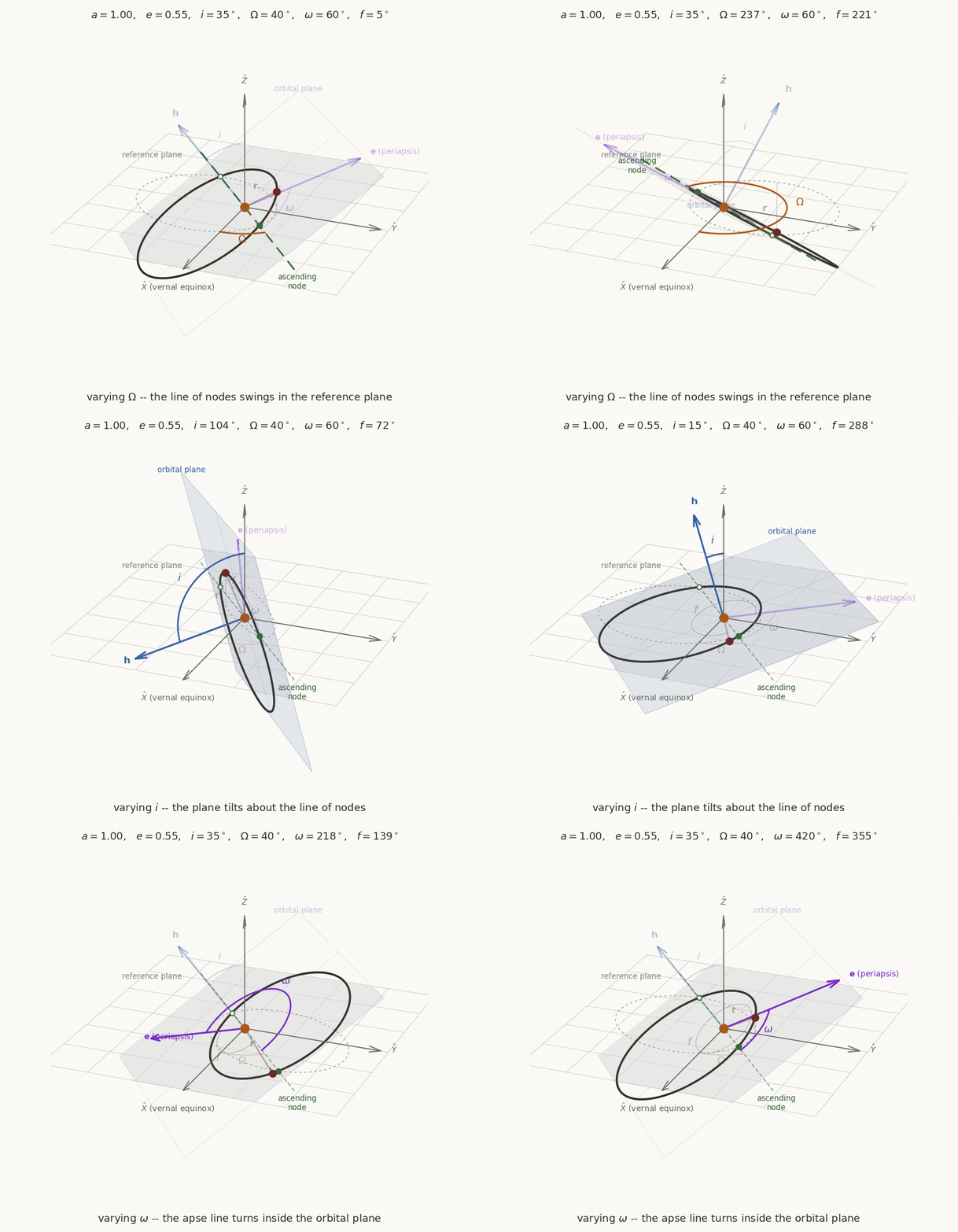
Which of the six elements can change the distance \(r\) of the body at a given true anomaly \(f\)? Which can change its speed?
Answer
Only \(a\) and \(e\) (through \(r=a(1-e^2)/(1+e\cos f)\) and vis-viva). Changing \(i\), \(\Omega\) or \(\omega\) moves the orbit rigidly: it cannot change any length or speed. Figure 4 is exactly this statement.4.3 Orbit classes by inclination
| \(i\) | name | remark |
|---|---|---|
| \(0^\circ\) | equatorial, prograde | no line of nodes |
| \(0^\circ<i<90^\circ\) | prograde (direct) | \(h_z>0\), moves eastward |
| \(90^\circ\) | polar | passes over both poles |
| \(90^\circ<i<180^\circ\) | retrograde | \(h_z<0\), moves westward |
| \(180^\circ\) | equatorial, retrograde | no line of nodes |
Two named cases are worth knowing. The Earth’s flattening (measured by the coefficient \(J_2=1.0826\times10^{-3}\); see the gravity note) makes the argument of periapsis drift at a rate proportional to \(5\cos^2i-1\). At the critical inclination \(i=63.4^\circ\) this vanishes, so the apogee stays put: Molniya orbits use it to keep their apogee over the northern hemisphere. The second case is the sun-synchronous orbit.
4.4 Sun-synchronous orbits
The same flattening also turns the orbital plane: the node drifts at
\[ \dot\Omega=-\frac32\,\frac{\sqrt\mu\,J_2R_\oplus^2}{(1-e^2)^2a^{7/2}}\,\cos i . \tag{1}\]
A satellite whose plane turns at exactly the rate at which the Sun moves round the sky,
\[ \dot\alpha_\odot=\frac{360^\circ}{365.2422\ \text{days}}=0.9856^\circ\ \text{per day, eastward}, \]
keeps the same orientation relative to the Sun all year (Figure 5). Such an orbit is called sun-synchronous: it crosses each latitude at the same local solar time on every pass.
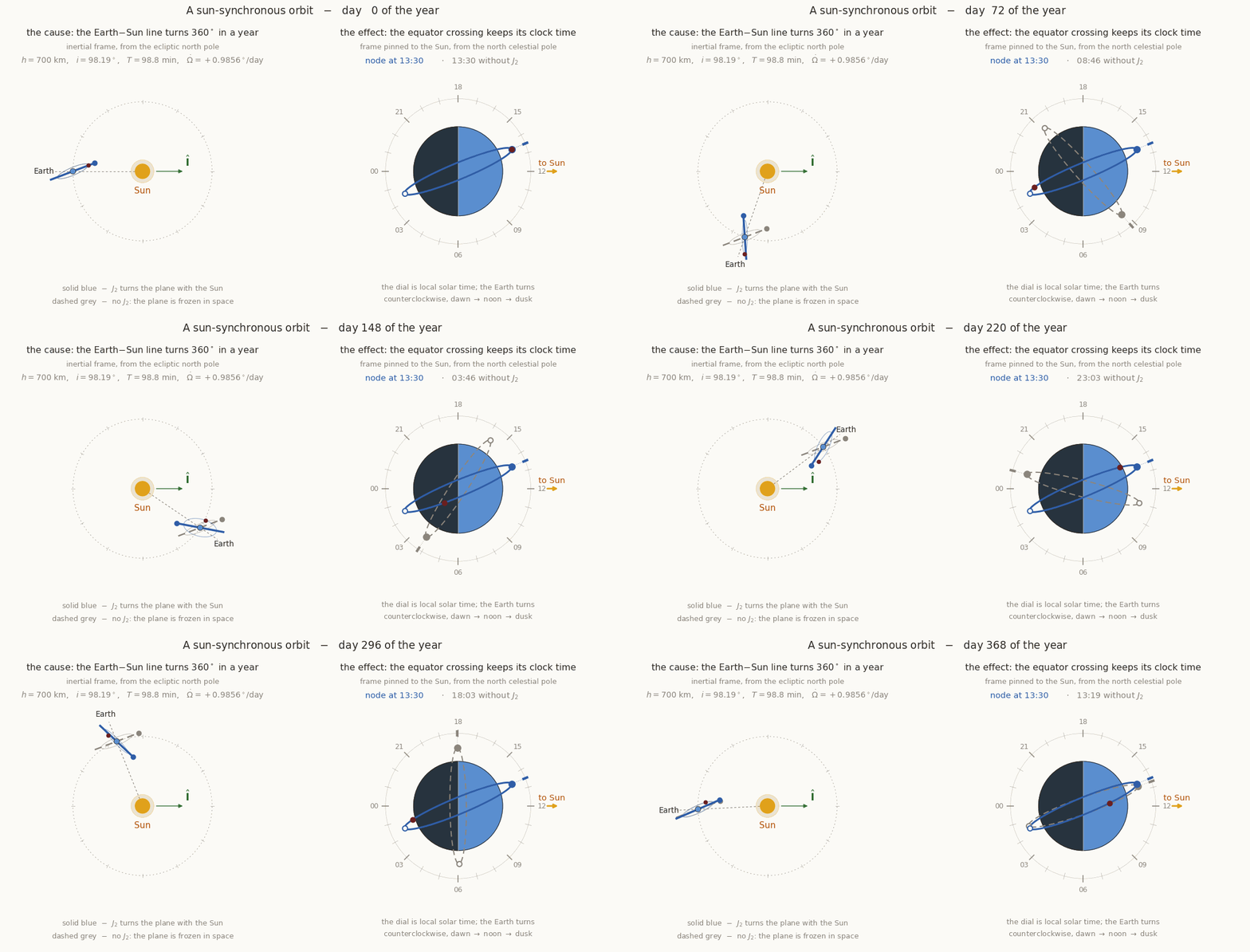
In Equation 1, everything except \(\cos i\) is positive. What sign must \(\cos i\) have for a sun-synchronous orbit? What does that say about the inclination?
Answer
The node must move eastward, \(\dot\Omega>0\), so \(\cos i<0\), i.e. \(i>90^\circ\). Every sun-synchronous orbit is retrograde. That is where the familiar \(i\approx98^\circ\) comes from; it is not a convention.Since \(\dot\Omega\) is linear in \(\cos i\), setting \(\dot\Omega=\dot\alpha_\odot\) gives the inclination directly:
\[ \boxed{\;\cos i=-\frac{2\,\dot\alpha_\odot\,(1-e^2)^2a^{7/2}}{3\sqrt\mu\,J_2R_\oplus^2}.\;} \]
Compute the sun-synchronous inclination and the period of circular orbits at \(400\), \(800\) and \(1200\) km altitude. (Convert \(\dot\alpha_\odot\) to rad/s.) Then find the altitude at which the right-hand side reaches \(-1\).
What you should find
| altitude | \(a\) [km] | \(i\) | \(T\) [min] |
|---|---|---|---|
| \(400\) km | \(6778.1\) | \(97.03^\circ\) | \(92.6\) |
| \(600\) km | \(6978.1\) | \(97.79^\circ\) | \(96.7\) |
| \(800\) km | \(7178.1\) | \(98.60^\circ\) | \(100.9\) |
| \(1000\) km | \(7378.1\) | \(99.48^\circ\) | \(105.1\) |
| \(1200\) km | \(7578.1\) | \(100.42^\circ\) | \(109.4\) |
What it buys. The same sunlight on every pass: the same Sun elevation in every image, so pictures taken years apart are comparable (Landsat and Sentinel-2 fly such orbits); a thermal and solar-array geometry that never drifts; and a free choice of the local time itself, about \(10{:}30\) for optical imaging, or a dawn–dusk orbit (\(06{:}00/18{:}00\)) for radar satellites that want their solar panels always lit. What it costs. The inclination is spent: it cannot also be chosen for coverage, and a retrograde launch gives up the eastward boost from the Earth’s rotation (about \(0.46\) km/s at the equator) that a due-east launch gets for free.
Is a satellite in a \(13{:}30\) sun-synchronous orbit always in sunlight?
Answer
No. “Sun-synchronous” fixes the angle between the orbital plane and the Sun, not the satellite’s illumination. A \(13{:}30\) orbit passes through the Earth’s shadow on every revolution. Only the dawn–dusk orbit, whose plane is nearly perpendicular to the Earth–Sun line, avoids eclipses, and even it does so only for part of the year.4.5 When the elements break down
Two of the orientation angles are measured from directions that can cease to exist.
- Circular orbit, \(e=0\). Then \(\mathbf e=\mathbf 0\): there is no periapsis, so \(\omega\) and \(f\) are both undefined. Their sum is not: the argument of latitude \(u=\omega+f\), the angle from the ascending node to the body, with \(\cos u=\mathbf n\cdot\mathbf r/(nr)\) and \(u>180^\circ\) if \(z<0\).
- Equatorial orbit, \(i=0^\circ\) or \(180^\circ\). Then \(\mathbf n=\mathbf 0\): there is no node, so \(\Omega\) and \(\omega\) are undefined, but the longitude of periapsis \(\varpi=\Omega+\omega\) is not, with \(\cos\varpi=e_I/e\) and \(\varpi>180^\circ\) if \(e_J<0\).
- Both: use the true longitude \(\lambda=\Omega+\omega+f\), with \(\cos\lambda=r_I/r\) and \(\lambda>180^\circ\) if \(r_J<0\).
These are legitimate only because the angle between the two planes in which their pieces are measured has collapsed to zero. Numerically the trouble starts before the exact degeneracy: for small \(e\) the direction of \(\mathbf e\) is poorly determined, and for small \(i\) the direction of \(\mathbf n\) is. Software either tests for it (\(e<10^{-8}\), \(\sin i<10^{-8}\)) or uses a non-singular set such as the equinoctial elements \(\left(a,\ e\cos\varpi,\ e\sin\varpi,\ \tan\tfrac i2\cos\Omega,\ \tan\tfrac i2\sin\Omega,\ \text{a longitude}\right)\), singular only for \(i=180^\circ\).
4.6 The elements at a glance
| element | what it fixes | constant in the two-body problem? | |
|---|---|---|---|
| size | \(a\) | the energy, \(\varepsilon=-\mu/2a\) | yes |
| shape | \(e\) | the type and flattening of the conic | yes |
| \(i\) | tilt of the plane | yes | |
| orientation | \(\Omega\) | swing of the plane about \(\hat{\mathbf K}\) | yes |
| \(\omega\) | turn of the apse line in the plane | yes | |
| position | \(f\) (or \(M\), or \(t_p\)) | where the body is | no |
Only the last runs with time. Under perturbations (\(J_2\), drag, the Sun and Moon) the first five drift slowly, which is why this set is the natural language of perturbation theory: the fast variable is isolated in one coordinate.
5 From \((\mathbf r,\mathbf v)\) to the elements
5.1 The algorithm
Tracking gives a state vector; catalogues want elements. Given \(\mathbf r\), \(\mathbf v\) in \(\{\hat{\mathbf I},\hat{\mathbf J},\hat{\mathbf K}\}\) and \(\mu\):
| # | quantity | formula | quadrant test |
|---|---|---|---|
| 1 | radius, speed | \(r=\lvert\mathbf r\rvert\), \(v=\lvert\mathbf v\rvert\) | |
| 2 | radial speed | \(v_r=\mathbf r\cdot\mathbf v/r\) | (used in 9) |
| 3 | angular momentum | \(\mathbf h=\mathbf r\times\mathbf v\), \(h=\lvert\mathbf h\rvert\) | |
| 4 | inclination | \(i=\arccos(h_K/h)\) | none needed |
| 5 | node vector | \(\mathbf n=\hat{\mathbf K}\times\mathbf h=(-h_J,\,h_I,\,0)\) | |
| 6 | RAAN | \(\Omega=\arccos(n_I/n)\) | if \(n_J<0\): \(\Omega\to360^\circ-\Omega\) |
| 7 | eccentricity | \(\mathbf e=\frac1\mu\left[\left(v^2-\frac\mu r\right)\mathbf r-(\mathbf r\cdot\mathbf v)\mathbf v\right]\) | |
| 8 | argument of periapsis | \(\omega=\arccos\frac{\mathbf n\cdot\mathbf e}{ne}\) | if \(e_K<0\): \(\omega\to360^\circ-\omega\) |
| 9 | true anomaly | \(f=\arccos\frac{\mathbf e\cdot\mathbf r}{er}\) | if \(v_r<0\): \(f\to360^\circ-f\) |
| 10 | size | \(a=\left(\frac2r-\frac{v^2}\mu\right)^{-1}\), \(p=\frac{h^2}\mu\) |
Show that the formula in step 7 is the same as \(\mathbf e=\mathbf v\times\mathbf h/\mu-\hat{\mathbf r}\). (Expand \(\mathbf v\times(\mathbf r\times\mathbf v)\).)
What you should find
\(\mathbf v\times(\mathbf r\times\mathbf v)=v^2\mathbf r-(\mathbf r\cdot\mathbf v)\mathbf v\), so \(\mathbf e=\frac1\mu\left[v^2\mathbf r-(\mathbf r\cdot\mathbf v)\mathbf v\right]-\frac{\mathbf r}r\), and \(\frac{\mathbf r}r=\frac1\mu\frac\mu r\mathbf r\). The form in the table needs no cross product, which is convenient by hand.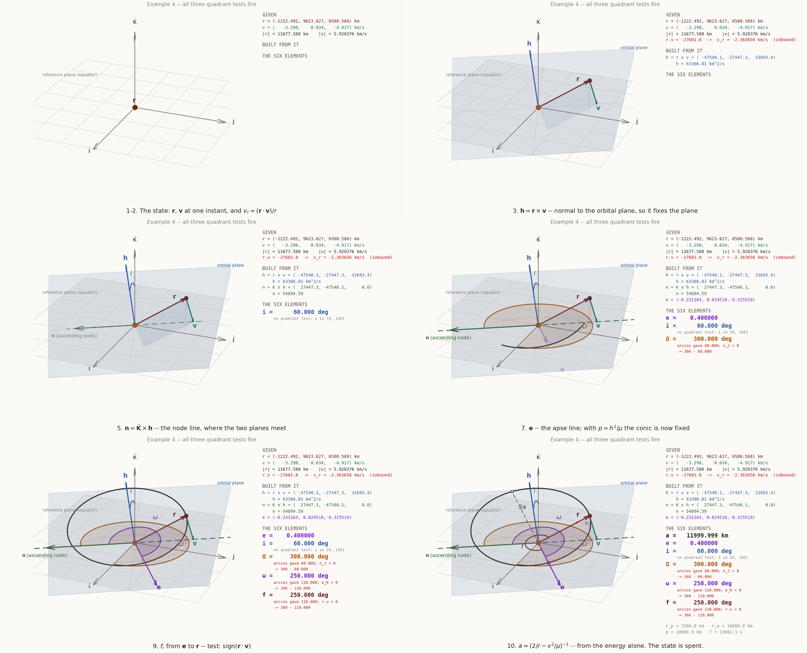
Steps 4, 6, 8 and 9 produce the four angles, and three of the four carry a quadrant test. Where do the tests come from, and why does \(i\) escape?
5.2 Why \(\arccos\) is not enough
Every angle in the table comes from a dot product, i.e. from its cosine. But \(\cos\theta=\cos(360^\circ-\theta)\), and \(\arccos\) always returns the answer in \([0^\circ,180^\circ]\). It cannot tell \(\theta\) from \(360^\circ-\theta\).
To decide, we need one more bit of information: the sign of the sine. For an angle measured from \(\mathbf a\) to \(\mathbf b\) about a unit axis \(\hat{\mathbf k}\) (with both vectors perpendicular to \(\hat{\mathbf k}\)),
\[ \cos\theta=\frac{\mathbf a\cdot\mathbf b}{ab},\qquad\sin\theta=\frac{(\mathbf a\times\mathbf b)\cdot\hat{\mathbf k}}{ab}. \]
So for each angle, compute that triple product and keep its sign. We now show that in every case it reduces to a single number we already have.
\(i\) needs no test, for a definitional reason. The inclination is defined on \([0^\circ,180^\circ]\), and on that interval \(\sin i\ge0\), so the sign of the sine carries no information. (The price is that \(i\) itself must carry the distinction between eastward and westward orbits, and \(\Omega\) must run over the full circle.) Note also that \(n=|\hat{\mathbf K}\times\mathbf h|=h\sin i\ge0\).
\(\Omega\): the sign of \(n_J\). \(\mathbf n\) lies in the equatorial plane, at angle \(\Omega\) from \(\hat{\mathbf I}\), so \(\mathbf n=n(\cos\Omega,\sin\Omega,0)\) and \(\sin\Omega=n_J/n\). Since \(n>0\),
\[ \boxed{\;\operatorname{sign}(\sin\Omega)=\operatorname{sign}(n_J),\qquad\Omega=\operatorname{atan2}(n_J,\ n_I).\;} \]
Find the corresponding tests for \(\omega\) and \(f\). For \(\omega\), measured from \(\mathbf n\) to \(\mathbf e\) about \(\hat{\mathbf h}\), compute \((\mathbf n\times\mathbf e)\cdot\hat{\mathbf h}\) using \(\mathbf n=\hat{\mathbf K}\times\mathbf h\) and \(\mathbf h\cdot\mathbf e=0\). For \(f\), measured from \(\mathbf e\) to \(\mathbf r\), compute \((\mathbf e\times\mathbf r)\cdot\hat{\mathbf h}\) using the definition of \(\mathbf e\) and \(\mathbf h\cdot\mathbf r=0\).
What you should find
With \((\mathbf A\times\mathbf B)\times\mathbf C=\mathbf B(\mathbf A\cdot\mathbf C)-\mathbf A(\mathbf B\cdot\mathbf C)\),
\[ \mathbf n\times\mathbf e=(\hat{\mathbf K}\times\mathbf h)\times\mathbf e=\mathbf h\,(\hat{\mathbf K}\cdot\mathbf e)-\hat{\mathbf K}\,(\mathbf h\cdot\mathbf e)=e_K\,\mathbf h, \]
so \(\sin\omega=he_K/(ne)=e_K/(e\sin i)\): the sign of \(e_K\). Periapsis is north of the equator exactly when \(\omega<180^\circ\).
The \(\hat{\mathbf r}\) part of \(\mathbf e\) contributes nothing to \(\mathbf e\times\mathbf r\), so
\[ \mathbf e\times\mathbf r=\frac{(\mathbf v\times\mathbf h)\times\mathbf r}{\mu}=\frac{\mathbf h(\mathbf v\cdot\mathbf r)-\mathbf v(\mathbf h\cdot\mathbf r)}{\mu}=\frac{\mathbf r\cdot\mathbf v}{\mu}\,\mathbf h, \]
so \(\sin f=h\,v_r/(\mu e)\): the sign of \(v_r\), i.e. of \(\mathbf r\cdot\mathbf v\). The body is past periapsis and climbing exactly when \(f<180^\circ\), which is the \(e\sin f\) in \(v_r=(\mu/h)e\sin f\).Collecting the three, with both arguments of each \(\operatorname{atan2}\) scaled consistently (\(\sin\) and \(\cos\) multiplied by the same positive number):
\[ \begin{aligned} \Omega&=\operatorname{atan2}\left(n_J,\ n_I\right),\\ \omega&=\operatorname{atan2}\left(\frac{e_K}{\sin i},\ \frac{\mathbf n\cdot\mathbf e}{n}\right),\\ f&=\operatorname{atan2}\left(\frac{h\,v_r}{\mu},\ \frac{\mathbf e\cdot\mathbf r}{r}\right). \end{aligned} \tag{2}\]
| angle | flip when | meaning |
|---|---|---|
| \(\Omega\) | \(n_J<0\) | ascending node in the half of the equator with \(J<0\) |
| \(\omega\) | \(e_K<0\) | periapsis south of the equator |
| \(f\) | \(\mathbf r\cdot\mathbf v<0\) | body inbound, falling towards periapsis |
In the \(f\) formula, why must the second argument be \(\mathbf e\cdot\mathbf r/r\) and not \(\mathbf e\cdot\mathbf r/e\)?
Answer
\(\operatorname{atan2}(y,x)\) returns the angle of the point \((x,y)\), so \(y\) and \(x\) must be \(\sin f\) and \(\cos f\) times the same positive factor. \(hv_r/\mu=e\sin f\), and \(\mathbf e\cdot\mathbf r/r=e\cos f\): both are scaled by \(e\). With \(\mathbf e\cdot\mathbf r/e=r\cos f\) instead, the point would be \((r\cos f,\ e\sin f)\), whose angle is not \(f\). The quadrant would still be right, but the angle would be wrong. (The same care applies to \(\omega\): \(e_K/\sin i=e\sin\omega\) and \(\mathbf n\cdot\mathbf e/n=e\cos\omega\).)There is a second reason to prefer \(\operatorname{atan2}\): \(\arccos\) is ill-conditioned near \(0^\circ\) and \(180^\circ\). From \(\delta\theta=-\delta(\cos\theta)/\sin\theta\), an error \(\epsilon\) in the cosine becomes an error of order \(\sqrt{2\epsilon}\) in the angle as \(\theta\to0\). With \(\epsilon=10^{-16}\) (double precision) that is \(10^{-8}\) rad: half the significant digits lost. \(\operatorname{atan2}\) has no such loss, and it also survives a cosine that rounding has pushed just outside \([-1,1]\), where \(\arccos\) returns “not a number”.
5.3 The remaining elements
The scalars come straight from the integrals:
\[ \varepsilon=\frac{v^2}2-\frac\mu r,\qquad a=-\frac{\mu}{2\varepsilon},\qquad p=\frac{h^2}\mu,\qquad e=\sqrt{1-\frac pa}, \]
and, for an ellipse, \(r_p=a(1-e)\), \(r_a=a(1+e)\) and \(T=2\pi\sqrt{a^3/\mu}\). Some books (Curtis, for example) use \(h\) instead of \(a\) as the size element. That is the better choice near the parabola, where \(a\to\infty\) while \(h\) and \(p\) stay finite.
6 From the elements to \((\mathbf r,\mathbf v)\)
6.1 Build in the orbital plane, then rotate
The forward map is easier, and comes in two steps.
Step 1: the conic in its own plane. In the perifocal frame \(\{\hat{\mathbf p},\hat{\mathbf q},\hat{\mathbf w}\}\) (\(\hat{\mathbf p}\) towards periapsis, \(\hat{\mathbf w}\) along \(\mathbf h\); see the perifocal note) the two-body note gives
\[ \mathbf r_{PQW}=\frac{p}{1+e\cos f}\begin{bmatrix}\cos f\\ \sin f\\ 0\end{bmatrix},\qquad \mathbf v_{PQW}=\frac\mu h\begin{bmatrix}-\sin f\\ e+\cos f\\ 0\end{bmatrix}. \]
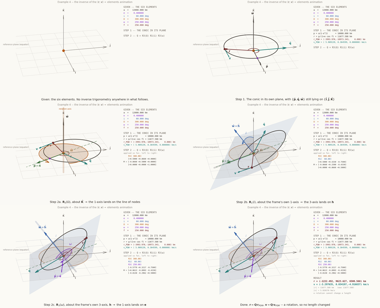
Step 2: rotate into the inertial frame. Undo the 3–1–3 sequence:
\[ \mathbf Q=\mathbf R_3(\Omega)\,\mathbf R_1(i)\,\mathbf R_3(\omega),\qquad \mathbf r=\mathbf Q\,\mathbf r_{PQW},\qquad\mathbf v=\mathbf Q\,\mathbf v_{PQW}, \]
where \(\mathbf R_1(\theta)\) and \(\mathbf R_3(\theta)\) rotate a vector by \(\theta\) about the first and third axes. Read the product from right to left: \(\omega\) turns \(\hat{\mathbf p}\) from the line of nodes to periapsis, \(i\) tilts the plane up from the equator about the line of nodes, and \(\Omega\) swings the line of nodes round from \(\hat{\mathbf I}\).
Multiplying out, with \(c_\theta=\cos\theta\) and \(s_\theta=\sin\theta\),
\[ \mathbf Q= \begin{bmatrix} c_\Omega c_\omega-s_\Omega s_\omega c_i & -c_\Omega s_\omega-s_\Omega c_\omega c_i & s_\Omega s_i\\ s_\Omega c_\omega+c_\Omega s_\omega c_i & -s_\Omega s_\omega+c_\Omega c_\omega c_i & -c_\Omega s_i\\ s_\omega s_i & c_\omega s_i & c_i \end{bmatrix}. \tag{3}\]
Check Equation 3 in three ways. (a) The third column should be \(\hat{\mathbf h}\) in inertial components; why should it not contain \(\omega\)? (b) The third row holds the out-of-plane components of \(\hat{\mathbf p},\hat{\mathbf q},\hat{\mathbf w}\); what should happen to it when \(i=0\)? (c) What should \(\mathbf Q\) be when \(i=\Omega=\omega=0\)?
What you should find
- \((\sin\Omega\sin i,\ -\cos\Omega\sin i,\ \cos i)\), with no \(\omega\): turning the apse line inside the plane cannot move the plane’s normal. (b) Its first two entries carry \(\sin i\) and vanish, and the third is \(1\): for an equatorial orbit \(\hat{\mathbf p}\) and \(\hat{\mathbf q}\) lie in the equator. (c) The identity matrix. \(\mathbf Q\) is orthogonal, \(\mathbf Q^{-1}=\mathbf Q^{\mathsf T}\), with \(\det\mathbf Q=+1\).
The forward map has no quadrant problem: it uses only sines and cosines of known angles, with no inverse trigonometry anywhere. All the difficulty of Section 5 came from inverting it. Together with Kepler’s equation, the two maps close the propagation loop:
\[ (\mathbf r,\mathbf v)_{t_0}\to(a,e,i,\Omega,\omega,f_0)\to M_0\to M(t)\to E\to f\to(\mathbf r,\mathbf v)_t , \]
in which only the last element changed. Five elements are the orbit; the sixth is the clock.
7 Worked examples
7.1 Example 1: from a state to the elements
Given \(\mathbf r=(-6045,\ -3490,\ 2500)\) km and \(\mathbf v=(-3.457,\ 6.618,\ 2.533)\) km/s.
Run the algorithm yourself before reading the solution below. Keep six significant figures.
Steps 1–3. \(r=7414.319\) km, \(v=7.884470\) km/s, \(\mathbf r\cdot\mathbf v=4133.245\) km\(^2\)/s, so \(v_r=+0.557468\) km/s (outbound). Then
\[ \mathbf h=\mathbf r\times\mathbf v=(-25\,385.17,\ 6669.485,\ -52\,070.74)\ \text{km}^2/\text{s}, \]
with \(h=58\,311.67\) km\(^2\)/s.
Step 4. \(i=\arccos(-52\,070.74/58\,311.67)=\arccos(-0.892973)=153.249^\circ\). More than \(90^\circ\): the orbit is retrograde.
Steps 5–6. \(\mathbf n=(-h_J,\ h_I,\ 0)=(-6669.485,\ -25\,385.17,\ 0)\), \(n=26\,246.69\). \(\arccos(n_I/n)=\arccos(-0.254108)=104.721^\circ\). But \(n_J<0\), so the ascending node is in the half of the equator with \(J<0\), and \(\Omega=360^\circ-104.721^\circ=255.279^\circ\). (Directly: \(\operatorname{atan2}(-25\,385.17,\ -6669.485)=-104.721^\circ\equiv255.279^\circ\).)
Step 7. With \(v^2-\mu/r=62.16486-53.76084=8.40402\) km\(^2\)/s\(^2\),
\[ \mathbf e=\frac1\mu\left[8.40402\,\mathbf r-4133.245\,\mathbf v\right]=(-0.091605,\ -0.142207,\ 0.026444), \]
so \(e=0.171212\).
Step 8. \(\cos\omega=\mathbf n\cdot\mathbf e/(ne)=4220.92/(26\,246.69\times0.171212)=0.939284\), so \(\arccos=20.068^\circ\). Test: \(e_K>0\), periapsis is north of the equator, and \(\omega=20.068^\circ\) stands.
Step 9. \(\cos f=\mathbf e\cdot\mathbf r/(er)=1116.16/(0.171212\times7414.319)=0.879270\), so \(\arccos=28.446^\circ\); \(v_r>0\), so \(f=28.446^\circ\) stands.
Step 10. \(\varepsilon=31.08243-53.76084=-22.67841\) km\(^2\)/s\(^2\), so \(a=8788.10\) km.
\[ \boxed{\;\begin{aligned} &a=8788.10\ \text{km},\quad e=0.171212,\quad i=153.249^\circ,\\ &\Omega=255.279^\circ,\quad \omega=20.068^\circ,\quad f=28.446^\circ \end{aligned}\;} \]
Sanity-check the answer: is the perigee above the atmosphere, and is \(r_p<r<r_a\)?
Answer
\(r_p=a(1-e)=7283.46\) km (\(905\) km altitude), \(r_a=a(1+e)=10\,292.73\) km, and \(r=7414\) km lies between them, just past perigee as \(f=28^\circ\) says. Also \(p=h^2/\mu=8530.48\) km and \(T=8198.9\) s \(=2.28\) h.7.2 Example 2: back again
Take the six numbers just found and run the forward map. With \(p=8530.48\) km and \(f=28.446^\circ\),
\[ \mathbf r_{PQW}=\begin{bmatrix}6519.19\\ 3531.62\\ 0\end{bmatrix}\ \text{km},\qquad \mathbf v_{PQW}=\begin{bmatrix}-3.25600\\ 7.18076\\ 0\end{bmatrix}\ \text{km/s}. \]
Before rotating: what should \(|\mathbf r_{PQW}|\) and \(|\mathbf v_{PQW}|\) be?
Answer
\(7414.32\) km and \(7.88447\) km/s, the \(r\) and \(v\) of Example 1. A rotation cannot change a length.With \(c_\Omega=-0.254107\), \(s_\Omega=-0.967176\), \(c_i=-0.892973\), \(s_i=0.450111\), \(c_\omega=0.939284\), \(s_\omega=0.343140\), Equation 3 gives
\[ \mathbf Q=\begin{bmatrix} -0.535036 & -0.724029 & -0.435336\\ -0.830591 & 0.545011 & 0.114377\\ 0.154451 & 0.422782 & -0.892973 \end{bmatrix}, \]
and then \(\mathbf r=\mathbf Q\mathbf r_{PQW}=(-6045.00,\ -3490.01,\ 2500.00)\) km and \(\mathbf v=\mathbf Q\mathbf v_{PQW}=(-3.45700,\ 6.61800,\ 2.53300)\) km/s. The round trip closes to about \(10\) m in position, which is entirely the six-figure rounding: carried in double precision, the residual is below \(10^{-8}\) km. A round trip is the cheapest test that exercises all three quadrant rules at once.
7.3 Example 3: the cost of one dropped test
Suppose that in Example 1 we had trusted \(\arccos\) and kept \(\Omega=104.721^\circ\), with everything else right.
Run the forward map with \(\Omega=104.721^\circ\) and the other five elements of Example 1. How far is the result from the true \(\mathbf r\)? What is \(|\mathbf r|\)?
What you should find
\(\mathbf r=(3548.89,\ 6010.62,\ 2500.00)\) km instead of \((-6045,\ -3490,\ 2500)\) km: \(13\,502\) km away, nearly twice the orbital radius, on the other side of the Earth. Yet \(|\mathbf r|=7414.32\) km, and \(a\), \(e\), \(i\), \(f\) are all still exactly right.This is the signature of a quadrant error: every scalar checks out and the vector is nonsense. A change of \(\Omega\) rotates the whole orbit about \(\hat{\mathbf K}\), preserving every length and every angle within the orbit. No magnitude check can catch it; only a component-by-component comparison can.
7.4 Example 4: all three tests fire
Given \(\mathbf r=(-1222.492,\ 9623.627,\ 6500.568)\) km and \(\mathbf v=(-3.297635,\ 0.034197,\ -4.916837)\) km/s. Then \(r=11\,677.59\) km, \(v=5.920376\) km/s, \(\mathbf r\cdot\mathbf v=-27\,601.8\), so \(v_r=-2.363656\) km/s (inbound), and
\[ \begin{aligned} \mathbf h&=(-47\,540.11,\ -27\,447.29,\ 31\,693.40), & h&=63\,386.81,\\ \mathbf n&=(27\,447.29,\ -47\,540.11,\ 0), & n&=54\,894.59,\\ \mathbf e&=(-0.231164,\ 0.024510,\ -0.325519), & e&=0.4, \end{aligned} \]
and \(i=\arccos(h_K/h)=\arccos(0.5)=60.000^\circ\).
Compute \(\Omega\), \(\omega\) and \(f\), applying the quadrant tests. Then find \(a\), \(r_p\), \(r_a\) and \(T\).
What you should find
| angle | \(\cos\) | \(\arccos\) | test | value | corrected |
|---|---|---|---|---|---|
| \(\Omega\) | \(+0.500000\) | \(60.000^\circ\) | \(n_J\) | \(-47\,540<0\) | \(\mathbf{300.000^\circ}\) |
| \(\omega\) | \(-0.342020\) | \(110.000^\circ\) | \(e_K\) | \(-0.3255<0\) | \(\mathbf{250.000^\circ}\) |
| \(f\) | \(-0.342020\) | \(110.000^\circ\) | \(\mathbf r\cdot\mathbf v\) | \(-27\,602<0\) | \(\mathbf{250.000^\circ}\) |
The body is inbound at \(f=250^\circ\). How long until perigee?
Answer
Convert \(f\) to \(E\) with the quadrant-safe form \(E=2\operatorname{atan2}\left(\sqrt{1-e}\sin\frac f2,\ \sqrt{1+e}\cos\frac f2\right)=273.851^\circ\). (The plain \(\arctan\) of the half-angle ratio gives \(-86.15^\circ\): the same quadrant trap, one level down.) Then \(\sin E=-0.997742\) and \(M=E-e\sin E=273.851^\circ+22.867^\circ=296.718^\circ\) (the term \(e\sin E\) is in radians, \(0.399\) rad \(=22.867^\circ\)). Perigee is at \(M=360^\circ\), so \(\Delta t=(360-296.718)/360\times13\,082.3=2299.6\) s \(=38.3\) min.7.5 Example 5: a hyperbola, forward
The forward map does not care what conic it draws. Given \(h=80\,000\) km\(^2\)/s, \(e=1.4\), \(i=30^\circ\), \(\Omega=40^\circ\), \(\omega=60^\circ\), \(f=30^\circ\).
Find \(p\) and \(a\), then \(\mathbf r_{PQW}\), \(\mathbf v_{PQW}\), and the inertial \(\mathbf r\), \(\mathbf v\). Check the energy.
What you should find
\(p=h^2/\mu=16\,056.20\) km and \(a=p/(1-e^2)=-16\,725.20\) km (negative, as it must be). \(\mathbf r_{PQW}=(6284.96,\ 3628.62,\ 0)\) km, \(\mathbf v_{PQW}=(-2.49125,\ 11.29047,\ 0)\) km/s, and
\[ \begin{aligned} \mathbf r&=(-4039.90,\ 4814.56,\ 3628.62)\ \text{km},\\ \mathbf v&=(-10.3860,\ -4.7719,\ 1.7439)\ \text{km/s}. \end{aligned} \]
Then \(r=7257.25\) km, \(v=11.5621\) km/s, \(\varepsilon=v^2/2-\mu/r=+11.917\) km\(^2\)/s\(^2>0\) and \(v_\infty=\sqrt{2\varepsilon}=4.882\) km/s. Nothing in Section 6 had to change.8 Summary
- Six numbers, one of which moves: \((a,e)\) size and shape, \((i,\Omega,\omega)\) orientation, and \(f\) (or \(M\), or \(t_p\)) position.
- Angles are measured in the geocentric equatorial frame: \(\hat{\mathbf I}\) to the vernal equinox, \(\hat{\mathbf K}\) along the spin axis. Both move (precession, nutation), so every orbit needs a frame epoch (J2000, or the quasar-based ICRF) as well as a state epoch.
- Three vectors generate everything: \(\mathbf h\) the plane, \(\mathbf n=\hat{\mathbf K}\times\mathbf h\) the ascending node, \(\mathbf e\) the line of apsides.
- \(J_2\) turns the node at a rate \(\propto-\cos i\); sun-synchronous orbits match it to the Sun and are therefore retrograde.
- \(i\) never needs a quadrant test; \(\Omega\), \(\omega\), \(f\) always do, with the tests \(\operatorname{sign}(n_J)\), \(\operatorname{sign}(e_K)\), \(\operatorname{sign}(\mathbf r\cdot\mathbf v)\). Use \(\operatorname{atan2}\) with consistently scaled arguments (Equation 2).
- \(e\to0\) removes \(\omega\); \(i\to0\) removes \(\Omega\). Use \(u\), \(\varpi\), \(\lambda\) or equinoctial elements.
- The forward map, \(\mathbf r=\mathbf Q\mathbf r_{PQW}\) with \(\mathbf Q=\mathbf R_3(\Omega)\mathbf R_1(i)\mathbf R_3(\omega)\), is easy; all the difficulty is in the inverse. Test with a component-wise round trip.
Where this goes next. Ground tracks need \(\Omega\) against the rotating Earth. The Earth’s oblateness drifts exactly two elements, \(\Omega\) and \(\omega\) (the gravity note). Orbit determination produces \((\mathbf r,\mathbf v)\) from observations, and Section 5 turns it into a catalogue entry. Manoeuvres (manoeuvres note) are naturally described as changes of elements: a Hohmann transfer changes \(a\) and \(e\), a plane change \(i\) and \(\Omega\), an apse rotation \(\omega\) alone. Finally, a caution: TLEs quote the same six numbers (\(i\), \(\Omega\), \(e\), \(\omega\), \(M\) and the mean motion), but they are mean elements tied to the SGP4 propagator, not the osculating elements of this note, and feeding them to a two-body propagator is a common and expensive mistake.
9 Exercises
- Geostationary. What are the elements of a geostationary satellite above \(75^\circ\)E at a given instant? Which of them are undefined, and what would you quote instead?
- The ISS. The space station has \(i=51.6^\circ\). What is the highest latitude it flies over? Why can it not be reached from a launch site at latitude \(60^\circ\) without a plane change?
- State to elements. Find the elements of \(\mathbf r=(7000,\ 0,\ 0)\) km, \(\mathbf v=(0,\ 5,\ 5)\) km/s. Which angles are delicate, and why?
- The sign tests. Construct a state with \(n_J<0\), \(e_K>0\) and \(v_r<0\), compute its elements, and confirm with a round trip.
- Sun-synchronous design. For a \(700\) km circular sun-synchronous orbit, find \(i\). How many revolutions does it make per day? Is the ground track repeated after one day?
- Molniya. A Molniya orbit has a period of half a sidereal day and \(e=0.74\). Find \(a\), \(r_p\), \(r_a\), and explain why \(i=63.4^\circ\) is chosen.
- Rotation matrices. Show that \(\mathbf R_3(\Omega)\mathbf R_1(i)\mathbf R_3(\omega)\), applied to \((0,0,1)\), gives \(\hat{\mathbf h}\), and applied to \((1,0,0)\) gives the unit vector towards periapsis.
All the numbers in this note and the worked examples are checked by orbital-elements-verify.py.