Universal Variables
One anomaly and one Kepler equation for every conic: propagating a state, the Lagrange coefficients, and Lambert’s problem
1 Where we are going
The most common question in orbital mechanics is this one:
A spacecraft is at position \(\mathbf r_0\) with velocity \(\mathbf v_0\). Where is it, and how fast is it moving, a time \(\Delta t\) later?
The two-body note answers it, but in three different ways. On an ellipse we convert the state to elements, find the eccentric anomaly \(E\) and solve Kepler’s equation; on a hyperbola we use the hyperbolic anomaly \(H\) and the hyperbolic Kepler equation; on a parabola we use \(D=\tan(f/2)\) and Barker’s equation. Before we can even start, we must know which of the three we are on. That is awkward for three reasons.
- Branching. A program must test \(e<1\), \(e=1\) or \(e>1\), and the test \(e=1\) is never exactly true in floating-point arithmetic.
- Loss of precision near \(e=1\). Comets, escape trajectories and Lambert solutions near the parabola have \(e\approx1\), and there the elliptic and hyperbolic formulas lose digits (Section 6.4 shows how many).
- Elements we do not need. To move a state forward in time we compute \(a\), \(e\), \(\omega\) and \(f\), and then throw them away. For a near-circular orbit \(\omega\) and \(f\) are individually ill defined, even though the motion is perfectly regular.
The Lambert note met the same problems from the other side and asked for three things: one iteration variable defined for every conic, one time-of-flight equation that is smooth through \(e=1\), and an iteration range that does not have to be worked out from the geometry first. This note supplies all three. The idea is to replace time by a new independent variable, the universal anomaly \(\chi\), in which the radial motion becomes a linear equation with constant coefficients. Everything else follows from that one fact.
History. Measuring the motion with a clock that runs at a rate proportional to \(1/r\) goes back to Karl Sundman, who used the substitution \(dt=r\,d\tau\) in his 1912–13 solution of the three-body problem to remove the singularity at a collision (Sundman 1913). For the two-body problem the functions \(C\) and \(S\) of this note are named after the German astronomer Karl Stumpff (1895–1970). In the 1960s several authors, Battin among them (Battin 1964), wrote the two-body problem entirely in such a variable, and the formulation became the standard way to write propagators and Lambert solvers (Bate, Mueller, and White 1971; Battin 1999).
The plan:
- Section 2 collects what we need from earlier notes.
- Section 3 introduces \(\chi\) and shows that \(r(\chi)\) obeys \(r''+\alpha r=1\).
- Section 4 integrates the clock to get the universal Kepler equation, explains what \(\chi\) is on each conic, and shows how to solve the equation.
- Section 5 derives the Lagrange coefficients in universal variables, so that \(\mathbf r=F\,\mathbf r_0+G\,\mathbf v_0\) for any \(\Delta t\).
- Section 6 gives the propagation algorithm, two worked examples, and the precision test.
- Section 7 solves Lambert’s problem in universal variables and redoes Example 1 of the Lambert note.
| Symbol | Meaning |
|---|---|
| \(\mathbf r_0,\ \mathbf v_0\); \(r_0,\ v_0\) | position and velocity at the start, and their lengths |
| \(v_{r0}=\mathbf r_0\cdot\mathbf v_0/r_0\) | radial velocity at the start |
| \(\mathbf r,\ \mathbf v\); \(r\) | position and velocity a time \(\Delta t\) later; \(r=\lvert\mathbf r\rvert\) |
| \(\alpha=1/a\) | reciprocal of the semi-major axis (\(>0\) ellipse, \(=0\) parabola, \(<0\) hyperbola) |
| \(\chi\) | universal anomaly, \(\chi=0\) at the start; units km\(^{1/2}\) |
| \(z=\alpha\chi^2\) | the argument of the Stumpff functions (dimensionless) |
| \(C(z),\ S(z)\) | Stumpff functions, Equation 9 |
| \(\sigma_0=\mathbf r_0\cdot\mathbf v_0/\sqrt\mu=r_0v_{r0}/\sqrt\mu\) | a scaled radial velocity at the start |
| \((\ )'\) | derivative with respect to \(\chi\); a dot is a derivative with respect to \(t\) |
| \(F,\ G,\ \dot F,\ \dot G\) | Lagrange coefficients, \(\mathbf r=F\mathbf r_0+G\mathbf v_0\), \(\mathbf v=\dot F\mathbf r_0+\dot G\mathbf v_0\) |
| \(f\), \(E\), \(H\) | true, eccentric and hyperbolic anomalies (as in the two-body note) |
Throughout, \(\mu=398\,600.4418\ \mathrm{km^3/s^2}\) (the Earth).
2 What you need first
Energy, and the reciprocal semi-major axis. On any two-body orbit the energy per unit mass is
\[ \varepsilon=\frac{v^2}{2}-\frac{\mu}{r}=-\frac{\mu}{2a}. \tag{1}\]
Evaluated at the start, it gives the semi-major axis from the state vector alone. We shall always use its reciprocal,
\[ \alpha=\frac1a=\frac{2}{r_0}-\frac{v_0^2}{\mu}. \tag{2}\]
\(\alpha\) is finite for every orbit: positive on an ellipse, zero on a parabola (where \(a\) itself is infinite), negative on a hyperbola. Using \(\alpha\) instead of \(a\) is the first step towards formulas without branches.
Radial and transverse motion. Split the velocity into a radial part \(\dot r\) and a transverse part \(r\dot\theta\). With the angular momentum \(h=r^2\dot\theta\) constant,
\[ v^2=\dot r^2+\frac{h^2}{r^2}, \qquad \ddot r-\frac{h^2}{r^3}=-\frac{\mu}{r^2}. \tag{3}\]
The first is Pythagoras; the second is the radial component of \(\ddot{\mathbf r}=-\mu\mathbf r/r^3\), derived in the two-body note.
Radial velocity from the state. Differentiating \(r^2=\mathbf r\cdot\mathbf r\) gives \(r\dot r=\mathbf r\cdot\mathbf v\), so \(v_{r0}=\dot r(0)=\mathbf r_0\cdot\mathbf v_0/r_0\).
Lagrange coefficients. The motion stays in the plane of \(\mathbf r_0\) and \(\mathbf v_0\), and these two vectors form a basis of that plane. So every later state is a combination of them,
\[ \mathbf r=F\,\mathbf r_0+G\,\mathbf v_0,\qquad \mathbf v=\dot F\,\mathbf r_0+\dot G\,\mathbf v_0, \tag{4}\]
with scalar coefficients that depend on \(\Delta t\) (the Lambert note derives them in terms of the transfer angle). Conservation of angular momentum gives \(F\dot G-\dot FG=1\). Our job in Section 5 is to find \(F\) and \(G\) as functions of time.
3 A new clock: the universal anomaly
3.1 Why change the clock?
On an eccentric orbit, almost all the turning happens in a short time near periapsis, and almost nothing happens for a long time near apoapsis. Measured in time, the motion is very uneven. A variable that runs fast where \(r\) is small and slowly where \(r\) is large spreads it out evenly. The simplest such variable is defined by
\[ \frac{d\chi}{dt}=\frac{\sqrt\mu}{r},\qquad \chi=0\ \text{at}\ t=t_0 . \tag{5}\]
The factor \(\sqrt\mu\) is there only to give \(\chi\) convenient units, km\(^{1/2}\). Because \(r>0\), \(\chi\) increases steadily with \(t\), so it is a legitimate clock: each instant has one value of \(\chi\) and each \(\chi\) one instant.
Derivatives with respect to \(\chi\) are written with a prime. By the chain rule,
\[ \frac{d}{dt}=\frac{d\chi}{dt}\,\frac{d}{d\chi}=\frac{\sqrt\mu}{r}\,\frac{d}{d\chi}, \qquad\text{equivalently}\qquad (\ )'=\frac{r}{\sqrt\mu}\,\dot{(\ )} . \tag{6}\]
3.2 The radial equation becomes linear
Apply Equation 6 to the distance \(r\) itself. The first derivative is
\[ r'=\frac{r\dot r}{\sqrt\mu}=\frac{\mathbf r\cdot\mathbf v}{\sqrt\mu}. \]
Its value at the start is the scaled radial velocity of Table 1, \(r'(0)=\sigma_0\). Differentiate once more, again with Equation 6, and use the product rule on \(r\dot r\):
\[ r''=\frac{r}{\sqrt\mu}\,\frac{d}{dt}\Bigl(\frac{r\dot r}{\sqrt\mu}\Bigr) =\frac{r}{\mu}\bigl(\dot r^2+r\ddot r\bigr). \]
Now evaluate the bracket with Equation 3. From the first equation and Equation 1, \(\dot r^2=v^2-h^2/r^2=2\mu/r-\mu\alpha-h^2/r^2\). From the second, \(r\ddot r=-\mu/r+h^2/r^2\). Adding,
\[ \dot r^2+r\ddot r=\frac{2\mu}{r}-\mu\alpha-\frac{h^2}{r^2}-\frac{\mu}{r}+\frac{h^2}{r^2} =\frac{\mu}{r}-\mu\alpha . \]
The angular momentum has cancelled. Multiplying by \(r/\mu\):
\[ \boxed{\ r''+\alpha\,r=1\ } \tag{7}\]
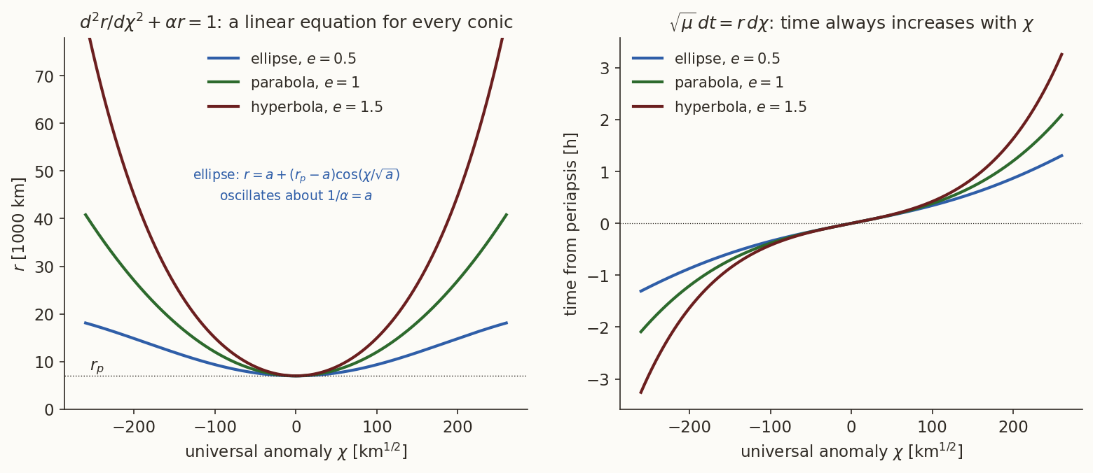
This is the central result of the note. In the time variable the radial motion obeys a nonlinear equation; in \(\chi\) it obeys the equation of a harmonic oscillator with a constant forcing, with constant coefficients, for every conic. The sign of \(\alpha\) only decides whether the free solution oscillates (\(\alpha>0\)), grows exponentially (\(\alpha<0\)), or is a polynomial (\(\alpha=0\)).
Why is it natural that the solution of Equation 7 oscillates about \(r=1/\alpha\) on an ellipse?
Answer
\(r=1/\alpha=a\) is the particular (constant) solution: \(0+\alpha\cdot a=1\). The free part oscillates about it with amplitude \(|r_0-a|\) (at periapsis start) between \(r_p=a(1-e)\) and \(r_a=a(1+e)\), which are equally far from \(a\), by \(ae\), on either side. So \(r(\chi)\) swings symmetrically about \(a\).3.3 Solving it, and the Stumpff functions
The initial conditions are \(r(0)=r_0\) and \(r'(0)=\sigma_0\).
Ellipse, \(\alpha>0\). The particular solution is \(1/\alpha\), and the free solutions are \(\cos\sqrt\alpha\,\chi\) and \(\sin\sqrt\alpha\,\chi\). Fitting the two initial conditions,
\[ r=\frac1\alpha+\Bigl(r_0-\frac1\alpha\Bigr)\cos\sqrt\alpha\,\chi+\frac{\sigma_0}{\sqrt\alpha}\sin\sqrt\alpha\,\chi . \tag{8}\]
Hyperbola, \(\alpha<0\): the same with \(\cos\to\cosh\), \(\sin\to\sinh\) and \(\sqrt\alpha\to\sqrt{-\alpha}\). Parabola, \(\alpha=0\): \(r''=1\) gives \(r=r_0+\sigma_0\chi+\chi^2/2\).
Three formulas again. To merge them, introduce \(z=\alpha\chi^2\) and the Stumpff functions
\[ C(z)=\frac{1-\cos\sqrt z}{z},\qquad S(z)=\frac{\sqrt z-\sin\sqrt z}{\bigl(\sqrt z\bigr)^{3}} , \tag{9}\]
read with \(\cos\sqrt z=\cosh\sqrt{-z}\) and \(\sin\sqrt z/\sqrt z=\sinh\sqrt{-z}/\sqrt{-z}\) when \(z<0\). Their Taylor series follow from those of \(\cos\) and \(\sin\),
\[ C(z)=\frac12-\frac{z}{24}+\frac{z^2}{720}-\cdots=\sum_{k\ge0}\frac{(-z)^k}{(2k+2)!}, \qquad S(z)=\frac16-\frac{z}{120}+\frac{z^2}{5040}-\cdots=\sum_{k\ge0}\frac{(-z)^k}{(2k+3)!}. \tag{10}\]
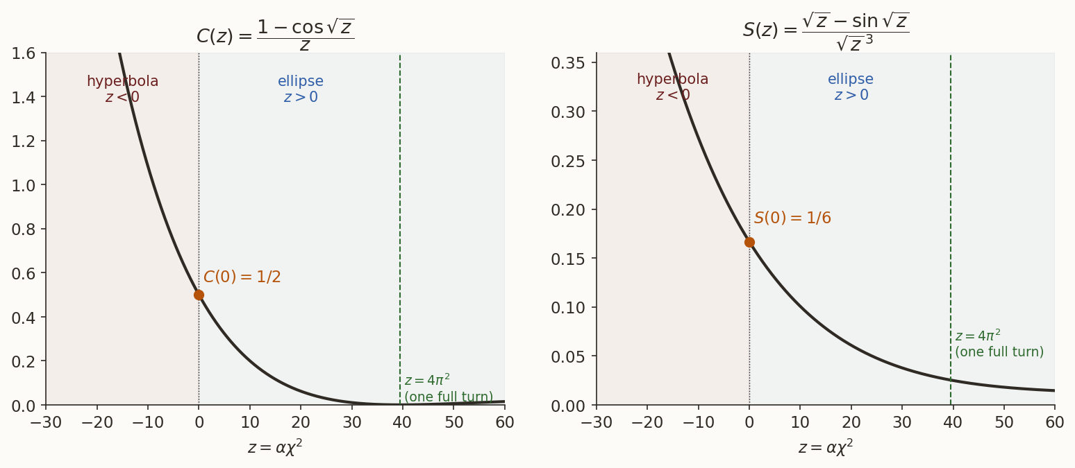
The series contain only integer powers of \(z\) and converge for every real \(z\). So \(C\) and \(S\) are smooth functions of \(z\) across \(z=0\), with \(C(0)=\tfrac12\) and \(S(0)=\tfrac16\) (Figure 1). There is no separate case for the parabola.
Use the series of \(\cos x\) and \(\sin x\) to derive Equation 10. Then explain why, in a program, you should switch to the series when \(|z|\) is small.
What you should find
\(1-\cos\sqrt z=z/2!-z^2/4!+\cdots\), so \(C=1/2!-z/4!+\cdots\); \(\sqrt z-\sin\sqrt z=z^{3/2}/3!-z^{5/2}/5!+\cdots\), so \(S=1/3!-z/5!+\cdots\). For small \(|z|\), \(1-\cos\sqrt z\) subtracts two numbers both close to \(1\): with \(z=10^{-6}\) the difference is \(5\times10^{-7}\), and about six of the sixteen significant digits are lost. The series has no such cancellation. _uv.py uses it for \(|z|<0.1\).Three identities, each a line of trigonometry, turn Equation 8 into Stumpff form. With \(z=\alpha\chi^2\):
\[ \cos\sqrt\alpha\,\chi=1-zC,\qquad \frac{\sin\sqrt\alpha\,\chi}{\sqrt\alpha}=\chi\,(1-zS),\qquad \frac{1-\cos\sqrt\alpha\,\chi}{\alpha}=\chi^2C . \tag{11}\]
(For the first, \(zC=1-\cos\sqrt z\) and \(\sqrt z=\sqrt\alpha\,\chi\). For the second, \(zS=1-\sin\sqrt z/\sqrt z\). The third is the definition of \(C\) multiplied by \(\chi^2\).) Substituting into Equation 8 and collecting \(1/\alpha\) terms, \(\tfrac1\alpha-\tfrac1\alpha(1-zC)=\tfrac{zC}{\alpha}=\chi^2C\):
\[ \boxed{\ r=\chi^2C(z)+\sigma_0\,\chi\,\bigl(1-zS(z)\bigr)+r_0\,\bigl(1-zC(z)\bigr)\ } \tag{12}\]
The hyperbolic and parabolic formulas give the same expression, because the identities hold for \(z<0\) with hyperbolic functions and, through the series, at \(z=0\). One formula, every conic.
Three derivatives will be needed repeatedly. They follow from Equation 11 by differentiating the trigonometric forms:
\[ \frac{d}{d\chi}\bigl[\chi^3S\bigr]=\chi^2C,\qquad \frac{d}{d\chi}\bigl[\chi^2C\bigr]=\chi(1-zS),\qquad \frac{d}{d\chi}\bigl[\chi(1-zS)\bigr]=1-zC . \tag{13}\]
(For example, \(\chi(1-zS)=\sin(\sqrt\alpha\chi)/\sqrt\alpha\) has derivative \(\cos\sqrt\alpha\chi=1-zC\). For the first, \(\chi^3S=(\chi-\sin(\sqrt\alpha\chi)/\sqrt\alpha)/\alpha\).)
4 The universal Kepler equation
4.1 Integrating the clock
Equation 5 says \(\sqrt\mu\,dt=r\,d\chi\). Integrate from the start (\(\chi=0\)) to \(\chi\), using 1 and the derivatives Equation 13 read backwards (\(\int\chi^2C\,d\chi=\chi^3S\), \(\int\chi(1-zS)\,d\chi=\chi^2C\), \(\int(1-zC)\,d\chi=\chi(1-zS)\)):
\[ \sqrt\mu\,\Delta t=\chi^3S+\sigma_0\chi^2C+r_0\,\chi\,(1-zS). \]
Since \(r_0\chi(1-zS)=r_0\chi-r_0\alpha\chi^3S\), the first and last terms combine:
\[ \boxed{\ \sqrt\mu\,\Delta t=\frac{r_0v_{r0}}{\sqrt\mu}\,\chi^2C(z)+\bigl(1-\alpha r_0\bigr)\,\chi^3S(z)+r_0\,\chi\ } \tag{14}\]
This is the universal Kepler equation. Given the start state and \(\Delta t\), it has one unknown, \(\chi\). And by construction its derivative is the distance:
\[ \frac{d(\sqrt\mu\,\Delta t)}{d\chi}=r(\chi)>0 . \tag{15}\]
So \(\Delta t\) is a strictly increasing function of \(\chi\), and every \(\Delta t\), positive or negative, has exactly one \(\chi\).
The two-body note writes the universal Kepler equation measured from periapsis, as \(\sqrt\mu\,(t-t_p)=r_p\chi+(1-r_p/a)\chi^3S\). Show that Equation 14 reduces to it.
Answer
At periapsis \(r_0=r_p\) and \(v_{r0}=0\), so the \(\chi^2C\) term vanishes and \(1-\alpha r_0=1-r_p/a\).4.2 What \(\chi\) is on each conic
\(\chi\) is not a new physical angle. On each conic it is the familiar anomaly, rescaled.
Ellipse. From the two-body note, \(r=a(1-e\cos E)\) and Kepler’s equation \(E-e\sin E=n(t-t_p)\) with \(n=\sqrt{\mu/a^3}\). Differentiating Kepler’s equation, \(\dot E(1-e\cos E)=n\), so \(\dot E=na/r\). Then
\[ \frac{d}{dt}\bigl(\sqrt a\,E\bigr)=\sqrt a\,\frac{na}{r}=\frac{\sqrt\mu}{r}, \]
which is Equation 5. Both start at zero change, so \(\chi=\sqrt a\,(E-E_0)\), and \(z=\alpha\chi^2=(E-E_0)^2\). The value \(z=4\pi^2\) in Figure 1 is one full revolution in \(E\).
Hyperbola. The same steps with \(r=a(1-e\cosh H)\) (where \(a<0\)) give \(\chi=\sqrt{-a}\,(H-H_0)\) and \(z=-(H-H_0)^2\).
Parabola. With \(D=\sqrt p\,\tan(f/2)\), \(r=p/(2\cos^2(f/2))\) and \(\dot f=\sqrt{\mu p}/r^2\): \(\dot D=\tfrac12\sqrt p\sec^2(f/2)\,\dot f=\sqrt p\,(r/p)\sqrt{\mu p}/r^2=\sqrt\mu/r\). So \(\chi=\sqrt p\,\bigl(\tan\tfrac f2-\tan\tfrac{f_0}{2}\bigr)\), Barker’s variable.
Figure 2 shows \(r(\chi)\) and \(t(\chi)\) for three orbits with the same periapsis. In \(\chi\) the ellipse is a cosine, the parabola a parabola and the hyperbola a hyperbolic cosine, all solutions of Equation 7. The time is the area under \(r(\chi)\), divided by \(\sqrt\mu\).
4.3 Solving for \(\chi\)
Equation 14 cannot be solved for \(\chi\) in closed form, but it is ideal for Newton’s method. Write the residual as \(\Phi(\chi)=(\text{right-hand side of @eq-ukepler})-\sqrt\mu\,\Delta t\). By Equation 15, \(\Phi'(\chi)=r(\chi)\), which 1 gives at no extra cost. Newton’s step is
\[ \chi_{k+1}=\chi_k-\frac{\Phi(\chi_k)}{r(\chi_k)} . \tag{16}\]
Because \(\Phi\) is increasing, there is exactly one root, and Newton’s method converges from any reasonable start.
Starting values. A good start saves iterations.
- Ellipse: \(\chi=\sqrt a\,\Delta E\), and over a step \(\Delta E\approx n\Delta t\) on average. So \(\chi_0=\sqrt a\,n\,\Delta t=\sqrt\mu\,\alpha\,\Delta t\).
- Hyperbola: for long steps the growing exponential dominates. With \(k=\sqrt{-\alpha}\), for large \(\chi\) both \(\chi^2C=(\cosh k\chi-1)/k^2\) and \(\chi^3S=(\sinh k\chi-k\chi)/k^3\) behave like \(e^{k\chi}/(2k^2)\) and \(e^{k\chi}/(2k^3)\). Keeping only those terms in Equation 14 and solving the logarithm, \[ \chi_0=\sqrt{-a}\,\ln\frac{-2\mu\alpha\,\Delta t}{r_0v_{r0}+\sqrt{-\mu a}\,(1-\alpha r_0)} . \]
- Parabola: \(\chi_0=\sqrt\mu\,\Delta t/r_0\) (the first term of Equation 14).
5 The Lagrange coefficients in universal variables
We now want \(F\) and \(G\) in Equation 4 as functions of \(\chi\). The neat route is to find a linear equation for the vector \(\mathbf r(\chi)\), just as Equation 7 is a linear equation for \(r(\chi)\).
Step 1: the vector equation in \(\chi\). By Equation 6, \(\mathbf r'=r\mathbf v/\sqrt\mu\). Differentiate again, using \(\dot{\mathbf v}=-\mu\mathbf r/r^3\) and \(r'=r\dot r/\sqrt\mu\):
\[ \mathbf r''=\frac{r}{\sqrt\mu}\,\frac{d}{dt}\Bigl(\frac{r\mathbf v}{\sqrt\mu}\Bigr) =\frac{r}{\mu}\Bigl(\dot r\,\mathbf v-\frac{\mu\,\mathbf r}{r^2}\Bigr) =\frac{r'}{\sqrt\mu}\,\mathbf v-\frac{\mathbf r}{r}. \]
Replace \(\mathbf v\) by \(\sqrt\mu\,\mathbf r'/r\) and multiply by \(r\):
\[ r\,\mathbf r''-r'\,\mathbf r'+\mathbf r=\mathbf 0 . \tag{17}\]
The coefficients \(r\) and \(r'\) vary, so this is not yet what we want.
Step 2: differentiate once more. The derivative of Equation 17 is \(r'\mathbf r''+r\mathbf r'''-r''\mathbf r'-r'\mathbf r''+\mathbf r'=\mathbf 0\). The \(r'\mathbf r''\) terms cancel, leaving \(r\,\mathbf r'''+(1-r'')\,\mathbf r'=\mathbf 0\). By Equation 7, \(1-r''=\alpha r\), and dividing by \(r\):
\[ \boxed{\ \mathbf r'''+\alpha\,\mathbf r'=\mathbf 0\ } \tag{18}\]
A third-order linear equation with constant coefficients, for every conic.
Step 3: its general solution. Each component of \(\mathbf r\) solves \(u'''+\alpha u'=0\). Three independent solutions are \(1\), \(\sin(\sqrt\alpha\chi)/\sqrt\alpha\) and \((1-\cos\sqrt\alpha\chi)/\alpha\), which by Equation 11 are
\[ u_1=1,\qquad u_2=\chi(1-zS),\qquad u_3=\chi^2C . \]
They are chosen so that at \(\chi=0\) their values, first derivatives and second derivatives form the identity matrix: \(u_1=1\), \(u_2'=1\), \(u_3''=1\) there and all the others are zero (check with Equation 13). So the solution with given \(\mathbf r(0)\), \(\mathbf r'(0)\), \(\mathbf r''(0)\) is simply
\[ \mathbf r(\chi)=\mathbf r(0)\,u_1+\mathbf r'(0)\,u_2+\mathbf r''(0)\,u_3 . \]
Step 4: the initial values. \(\mathbf r(0)=\mathbf r_0\) and \(\mathbf r'(0)=r_0\mathbf v_0/\sqrt\mu\). From Equation 17 at \(\chi=0\), with \(r'(0)=\sigma_0\): \(\mathbf r''(0)=(\sigma_0\,\mathbf r'(0)-\mathbf r_0)/r_0=\sigma_0\mathbf v_0/\sqrt\mu-\mathbf r_0/r_0\). Therefore
\[ \mathbf r=\mathbf r_0+\frac{r_0\mathbf v_0}{\sqrt\mu}\,\chi(1-zS) +\Bigl(\frac{\sigma_0\mathbf v_0}{\sqrt\mu}-\frac{\mathbf r_0}{r_0}\Bigr)\chi^2C =\Bigl(1-\frac{\chi^2C}{r_0}\Bigr)\mathbf r_0 +\frac{r_0\chi(1-zS)+\sigma_0\chi^2C}{\sqrt\mu}\,\mathbf v_0 . \]
Step 5: read off \(F\) and \(G\). The coefficient of \(\mathbf r_0\) is \(F\). In the coefficient of \(\mathbf v_0\), the universal Kepler equation in the form before Equation 14 says \(r_0\chi(1-zS)+\sigma_0\chi^2C=\sqrt\mu\,\Delta t-\chi^3S\). Hence
\[ \boxed{\ F=1-\frac{\chi^2}{r_0}\,C(z),\qquad G=\Delta t-\frac{\chi^3}{\sqrt\mu}\,S(z)\ } \tag{19}\]
Step 6: the velocity coefficients. Differentiate in time, \(\dot{(\ )}=(\sqrt\mu/r)(\ )'\), using Equation 13 and \(\chi(1-zS)=\chi-\alpha\chi^3S\):
\[ \boxed{\ \dot F=\frac{\sqrt\mu}{r\,r_0}\bigl(\alpha\chi^3S(z)-\chi\bigr),\qquad \dot G=1-\frac{\chi^2}{r}\,C(z)\ } \tag{20}\]
where \(r\) is 1 (or \(\lvert F\mathbf r_0+G\mathbf v_0\rvert\)).
On an ellipse, \(\chi=\sqrt a\,\Delta E\) (Section 4.2). Show that Equation 19 becomes the familiar elliptic form \(F=1-\frac{a}{r_0}(1-\cos\Delta E)\), \(G=\Delta t-\sqrt{a^3/\mu}\,(\Delta E-\sin\Delta E)\).
Answer
\(z=\alpha\chi^2=\Delta E^2\), so \(\chi^2C=a\,\Delta E^2\,(1-\cos\Delta E)/\Delta E^2=a(1-\cos\Delta E)\) and \(\chi^3S=a^{3/2}\Delta E^3(\Delta E-\sin\Delta E)/\Delta E^3=a^{3/2}(\Delta E-\sin\Delta E)\). Universal variables are not a new theory of the orbit; they are the same Lagrange coefficients, written so that one formula covers all three conics.Verify Equation 20. For \(\dot G\), differentiate \(G=\Delta t-\chi^3S/\sqrt\mu\) in time and use \(d(\chi^3S)/d\chi=\chi^2C\) from Equation 13.
What you should find
\(\dot G=1-\frac{1}{\sqrt\mu}\,\frac{\sqrt\mu}{r}\,\chi^2C=1-\chi^2C/r\). For \(\dot F\): \(\dot F=-\frac{1}{r_0}\,\frac{\sqrt\mu}{r}\,\chi(1-zS)=\frac{\sqrt\mu}{rr_0}(\alpha\chi^3S-\chi)\).Why must \(F\dot G-\dot FG=1\) hold, and how would you use it in a program?
Answer
It is conservation of angular momentum: \(\mathbf r\times\mathbf v=(F\dot G-\dot FG)\,\mathbf r_0\times\mathbf v_0\) (the Lambert note does the expansion). In a program it is a free accuracy check, or a way to get the fourth coefficient from the other three.6 Propagating a state
6.1 The algorithm
Given \(\mathbf r_0\), \(\mathbf v_0\) and \(\Delta t\) (which may be negative):
- \(r_0=\lvert\mathbf r_0\rvert\), \(v_{r0}=\mathbf r_0\cdot\mathbf v_0/r_0\), and \(\alpha=2/r_0-v_0^2/\mu\) (Equation 2).
- Solve Equation 14 for \(\chi\) by Newton’s method (Equation 16), from the starting value of Section 4.3.
- \(z=\alpha\chi^2\); evaluate \(C(z)\) and \(S(z)\) (the series for small \(|z|\)).
- \(F\) and \(G\) from Equation 19; \(\mathbf r=F\mathbf r_0+G\mathbf v_0\) and \(r=\lvert\mathbf r\rvert\).
- \(\dot F\) and \(\dot G\) from Equation 20; \(\mathbf v=\dot F\mathbf r_0+\dot G\mathbf v_0\).
No elements, no branches on the conic type, no anomalies. The code is _uv.py.
6.2 Example 1: three hours on a transfer orbit
Given. A satellite has, in the geocentric equatorial frame, \(\mathbf r_0=(-2757.4,\ -6465.5,\ -1726.8)\) km and \(\mathbf v_0=(7.4488,\ -4.3468,\ -4.4076)\) km/s. Find its state \(3\) hours later.
Step 1. \(r_0=7237.94\) km, \(v_0=9.6854\) km/s, \(v_{r0}=\mathbf r_0\cdot\mathbf v_0/r_0=2.0967\) km/s, and
\[ \alpha=\frac{2}{7237.94}-\frac{9.6854^2}{398\,600.44}=4.0983\times10^{-5}\ \mathrm{km^{-1}}, \]
positive, so an ellipse with \(a=1/\alpha=24\,400.5\) km. (The elements are not needed; for the record, \(e=0.72001\) and the satellite is at \(f_0=30.00^\circ\).)
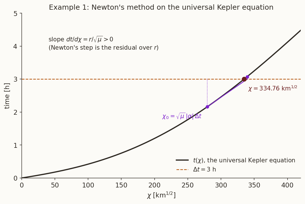
Step 2. \(\Delta t=10\,800\) s, and the starting value is \(\chi_0=\sqrt\mu\,\alpha\,\Delta t=279.443\) km\(^{1/2}\). Newton’s iterations (Figure 3):
| \(k\) | \(0\) | \(1\) | \(2\) | \(3\) | \(4\) |
|---|---|---|---|---|---|
| \(\chi_k\) [km\(^{1/2}\)] | \(279.443\) | \(339.352\) | \(334.779\) | \(334.757\) | \(334.757\) |
Step 3. \(z=\alpha\chi^2=4.5926\), so \(\sqrt z=2.143\) rad and \(C=0.33565\), \(S=0.13232\).
Steps 4 and 5.
\[ F=1-\frac{334.757^2\times0.33565}{7237.94}=-4.19676,\qquad G=10\,800-\frac{334.757^3\times0.13232}{\sqrt{398\,600.44}}=2937.580\ \mathrm s, \]
so \(\mathbf r=F\mathbf r_0+G\mathbf v_0=(33\,453.581,\ 14\,365.062,\ -5700.716)\) km, \(r=36\,850.99\) km. Then
\[ \dot F=-3.10843\times10^{-4}\ \mathrm{s^{-1}},\qquad \dot G=-0.020700, \]
and \(\mathbf v=(0.70292,\ 2.09973,\ 0.62800)\) km/s. The check \(F\dot G-\dot FG=1\) holds to twelve digits, and a direct numerical integration of \(\ddot{\mathbf r}=-\mu\mathbf r/r^3\) agrees to better than a millimetre.
What the numbers say. \(z=4.59\) means \(\Delta E=\sqrt z=2.143\) rad \(=122.79^\circ\): in three hours the eccentric anomaly advanced by \(122.79^\circ\), and the true anomaly went from \(30.00^\circ\) to \(161.08^\circ\). We never computed either.
6.3 Example 2: a day on an escape hyperbola
Given. The departure hyperbola of Example 1 of the patched-conics note: periapsis \(r_p=6678.137\) km, excess speed \(v_\infty=2.9447\) km/s, so \(v_p=\sqrt{v_\infty^2+2\mu/r_p}=11.3157\) km/s. Start at periapsis, \(\mathbf r_0=(6678.137,\ 0,\ 0)\) km, \(\mathbf v_0=(0,\ 11.3157,\ 0)\) km/s. Find the state one day later.
Steps 1–2. \(v_{r0}=0\) and \(\alpha=-2.1754\times10^{-5}\) km\(^{-1}\): a hyperbola with \(a=-45\,968\) km. The logarithmic start gives \(\chi_0=486.38\) km\(^{1/2}\), and Newton’s method takes six steps to \(\chi=571.733\) km\(^{1/2}\).
Steps 3–5. \(z=\alpha\chi^2=-7.1110\), negative, and the same formulas give \(F=-41.887\), \(G=16\,240.18\) s, \(r=334\,692\) km and \(v=3.3246\) km/s.
Checks. By Equation 1, the speed at \(334\,692\) km should be \(\sqrt{v_\infty^2+2\mu/r}=3.3246\) km/s. It is. And \(\chi/\sqrt{-a}=2.6666\) is the change in the hyperbolic anomaly: the true anomaly has reached \(146.70^\circ\), approaching the asymptote’s \(f_\infty=150.83^\circ\).
The patched-conics note says this spacecraft leaves the Earth’s sphere of influence (\(925\,000\) km) after about \(3.2\) days. Using the hyperbolic relation \(r=a(1-e\cosh H)\) with \(a=-45\,968\) km and \(e=1.1453\), find \(H\) at the sphere, then \(\chi=\sqrt{-a}\,H\), and check the time with Equation 14.
What you should find
\(\cosh H=(1+925\,000/45\,968)/1.1453=18.44\), so \(H=3.607\) and \(\chi=773.4\) km\(^{1/2}\). Then \(z=-13.01\) and Equation 14 gives \(\Delta t=2.73\times10^5\) s \(=3.16\) days.6.4 Why it matters: precision near \(e=1\)
How much do the classical formulas actually lose near the parabola? A test: take an orbit with periapsis \(7000\) km, start \(10\) minutes before periapsis, and step \(20\) minutes across it. Do this for eccentricities from \(e=0.9\) to \(1-10^{-9}\), and from \(1+10^{-9}\) to \(1.1\), and compare with the same calculation in \(50\)-digit arithmetic (Figure 4).
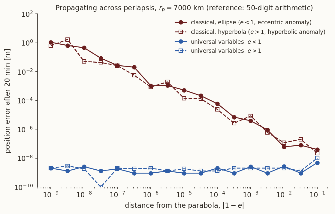
Where do the digits go? Near \(e=1\) the semi-major axis \(a=-\mu/2\varepsilon\) is computed from an energy that is a tiny difference of two large numbers, so \(a\) carries a large relative error; the mean motion \(n=\sqrt{\mu/a^3}\) and the factor \(\sqrt{(1-e)/(1+e)}\) inherit it; and in \(E-e\sin E\) for small \(E\) the two terms nearly cancel. The universal formulation never divides by \(1-e\), never forms \(a\), and evaluates \(C\) and \(S\) by a series where cancellation would occur. \(\alpha\) is small near the parabola, and a small \(\alpha\) is harmless.
7 Lambert’s problem in universal variables
7.1 The problem, and the plan
Given two positions \(\mathbf r_1\), \(\mathbf r_2\) and the time of flight \(\Delta t\), find the velocities \(\mathbf v_1\) and \(\mathbf v_2\). The transfer angle \(\Delta\theta\) from \(\mathbf r_1\) to \(\mathbf r_2\), in the direction of motion, follows from the geometry (the Lambert note explains how).
The Lambert note found the Lagrange coefficients in terms of the semi-latus rectum \(p\) and \(\Delta\theta\):
\[ F=1-\frac{r_2}{p}(1-\cos\Delta\theta),\quad G=\frac{r_1r_2\sin\Delta\theta}{\sqrt{\mu p}},\quad \dot G=1-\frac{r_1}{p}(1-\cos\Delta\theta), \tag{21}\]
\[ \dot F=\sqrt{\frac\mu p}\,\tan\frac{\Delta\theta}{2}\Bigl[\frac{1-\cos\Delta\theta}{p}-\frac1{r_1}-\frac1{r_2}\Bigr]. \tag{22}\]
Section 5 found the same four coefficients in terms of \(\chi\) and \(z\), with \(\mathbf r_0\to\mathbf r_1\) and \(\mathbf r\to\mathbf r_2\). Setting the two sets equal eliminates \(p\) and leaves one equation in one unknown, \(z\).
7.2 The derivation
Step 1: \(F\) fixes a combination of \(\chi\) and \(z\). Equating Equation 19 with Equation 21, \(\chi^2C/r_1=r_2(1-\cos\Delta\theta)/p\). Name the left-hand combination \(y\):
\[ y=\chi^2C(z)=\frac{r_1r_2(1-\cos\Delta\theta)}{p} . \tag{23}\]
(\(\dot G\) gives the same relation, a consistency check.) \(y\) has units of length, and \(y>0\) because \(p>0\).
Step 2: \(\dot F\) gives \(y\) as a function of \(z\). Write Equation 22 with \(1/p=y/[r_1r_2(1-\cos\Delta\theta)]\) from Equation 23. The bracket becomes \((y-r_1-r_2)/(r_1r_2)\), so
\[ \dot F=\sqrt\mu\,\sqrt{\frac{y}{r_1r_2(1-\cos\Delta\theta)}}\;\tan\frac{\Delta\theta}{2}\;\frac{y-r_1-r_2}{r_1r_2}. \]
The universal form Equation 20, with \(\chi(1-zS)=\chi-\alpha\chi^3S\), is \(\dot F=\sqrt\mu\,\chi\,(zS-1)/(r_1r_2)\), and \(\chi=\sqrt{y/C}\) by Equation 23. Equate the two, cancel \(\sqrt\mu\sqrt y/(r_1r_2)\) from both sides, and solve for \(y\):
\[ y=r_1+r_2+\frac{\sqrt{r_1r_2(1-\cos\Delta\theta)}}{\tan(\Delta\theta/2)}\;\frac{zS-1}{\sqrt C} . \]
The geometric factor simplifies with \(1-\cos\Delta\theta=2\sin^2(\Delta\theta/2)\). Define
\[ A=\sin\Delta\theta\,\sqrt{\frac{r_1r_2}{1-\cos\Delta\theta}}=\sqrt{2r_1r_2}\,\cos\frac{\Delta\theta}{2}, \tag{24}\]
a constant fixed by the geometry alone. Then
\[ \boxed{\ y(z)=r_1+r_2+A\,\frac{z\,S(z)-1}{\sqrt{C(z)}}\ } \tag{25}\]
Step 3: \(G\) gives the time of flight. From Equation 19, \(\sqrt\mu\,\Delta t=\chi^3S+\sqrt\mu\,G\). With \(\chi=\sqrt{y/C}\), \(\chi^3S=(y/C)^{3/2}S\). With Equation 21 and Equation 23, \(\sqrt\mu\,G=r_1r_2\sin\Delta\theta/\sqrt p=r_1r_2\sin\Delta\theta\,\sqrt y/\sqrt{r_1r_2(1-\cos\Delta\theta)}=A\sqrt y\). Therefore
\[ \boxed{\ \sqrt\mu\,\Delta t=\Bigl(\frac{y(z)}{C(z)}\Bigr)^{3/2}S(z)+A\,\sqrt{y(z)}\ } \tag{26}\]
One equation, one unknown \(z\), the same for every conic.
Step 4: the velocities. Once \(z\) is known, \(y\) follows from Equation 25, and Equation 23 turns the coefficients into
\[ F=1-\frac{y}{r_1},\qquad G=A\sqrt{\frac y\mu},\qquad \dot G=1-\frac{y}{r_2}, \tag{27}\]
and the Lambert note gives
\[ \mathbf v_1=\frac{\mathbf r_2-F\,\mathbf r_1}{G},\qquad \mathbf v_2=\frac{\dot G\,\mathbf r_2-\mathbf r_1}{G}. \tag{28}\]
7.3 The equation in \(z\)
Figure 5 plots \(y(z)\) and \(\Delta t(z)\) for the geometry of Example 3.
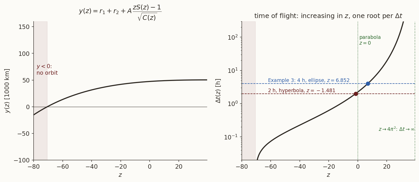
What the figure shows holds in general (for zero extra revolutions):
- The sign of \(z\) is the conic. \(z>0\) is an ellipse, \(z=0\) the parabola, \(z<0\) a hyperbola. So one evaluation of Equation 26 at \(z=0\) gives the parabolic time \(\Delta t_{\rm par}\), and tells us which side the answer is on, as the existence theorem of the Lambert note says.
- The range of \(z\) is simple. Above: \(z<4\pi^2\), since \(C(4\pi^2)=0\) makes \(\Delta t\) infinite (a full revolution). Below: on a short-way transfer, \(A>0\), and \(z\) must keep \(y(z)>0\). On a long-way transfer, \(A<0\), and since \(zS-1<0\) for every \(z\), \(y>0\) automatically.
- \(\Delta t(z)\) is increasing, so there is one root, and Newton’s method on \(z\) (with a step that is halved if it would leave the admissible range) converges.
These answer the three wishes of the Lambert note: one variable (\(z\)) for every conic, one equation (Equation 26) smooth through the parabola, and a range of iteration fixed by \(C(4\pi^2)=0\) and \(y>0\) instead of a geometry-dependent window.
7.4 Example 3: the Lambert note’s LEO-to-GEO transfer
Given (Example 1 of the Lambert note): \(\mathbf r_1=(6678.137,\ 0,\ 0)\) km, \(\mathbf r_2=42\,164\,(\cos175^\circ,\ \sin175^\circ,\ 0)\) km, \(\Delta t=4\) h \(=14\,400\) s.
Geometry. \(\Delta\theta=175^\circ\) (prograde, short way) and, by Equation 24, \(A=\sqrt{2\times6678.137\times42\,164}\,\cos87.5^\circ=1035.126\) km.
Which conic? At \(z=0\), \(C=\tfrac12\), \(S=\tfrac16\), \(y=r_1+r_2-A\sqrt2=47\,378.25\) km and Equation 26 gives \(\Delta t=2.238\) h, exactly the parabolic time \(\Delta t_{\rm par}\) of the Lambert note. Since \(4\) h is longer, the transfer is an ellipse and \(z>0\).
Newton on \(z\), starting from \(z=0\):
| step | \(z\) | \(y\) [km] | \(\Delta t\) [h] |
|---|---|---|---|
| 0 | \(0\) | \(47\,378.25\) | \(2.238033\) |
| 1 | \(10.18475\) | \(48\,878.56\) | \(5.553954\) |
| 2 | \(7.49666\) | \(48\,548.73\) | \(4.250411\) |
| 3 | \(6.87788\) | \(48\,466.49\) | \(4.009509\) |
| 4 | \(6.85248\) | \(48\,463.06\) | \(4.000015\) |
| 5 | \(6.85244\) | \(48\,463.06\) | \(4.000000\) |
Velocities. With \(y=48\,463.06\) km, Equation 27 gives
\[ F=1-\frac{48\,463.06}{6678.137}=-6.25697,\qquad G=1035.126\sqrt{\frac{48\,463.06}{398\,600.44}}=360.936\ \mathrm s,\qquad \dot G=1-\frac{48\,463.06}{42\,164}=-0.14939, \]
and Equation 28,
\[ \mathbf v_1=(-0.60573,\ 10.18142,\ 0)\ \mathrm{km/s},\qquad \mathbf v_2=(-1.11668,\ -1.52104,\ 0)\ \mathrm{km/s}. \]
These are the Lambert note’s values to every digit. The two methods also agree on the orbit: by Equation 23, \(p=r_1r_2(1-\cos\Delta\theta)/y=11\,598.163\) km, the root of the Lambert note’s \(p\)-iteration. Propagating \((\mathbf r_1,\mathbf v_1)\) for \(4\) h with the algorithm of Section 6.1 lands on \(\mathbf r_2\) to \(10^{-10}\) km.
Repeat Example 3 with \(\Delta t=2\) h (Example 2 of the Lambert note). Before computing, say whether \(z\) will be positive or negative, and why.
What you should find
\(2\) h is shorter than \(\Delta t_{\rm par}=2.238\) h, so the transfer is a hyperbola and \(z<0\). Newton converges to \(z=-1.4807\), and \(\mathbf v_1\) has \(y\)-component \(10.32782\) km/s; the orbit has \(e=1.1009\). The same equation, the same code, no branch.8 Summary
- The clock \(d\chi=\sqrt\mu\,dt/r\) turns the radial equation into \(r''+\alpha r=1\) (Equation 7), linear with constant coefficients, for every conic. \(\alpha=1/a=2/r_0-v_0^2/\mu\) is finite on a parabola.
- Its solution, written with the Stumpff functions \(C(z)\), \(S(z)\), \(z=\alpha\chi^2\), is
- \(C\) and \(S\) are entire functions; evaluate them by series near \(z=0\).
- Integrating the clock gives the universal Kepler equation Equation 14, whose derivative in \(\chi\) is \(r>0\): one root for every \(\Delta t\), found by Newton’s method with step \(\Phi/r\).
- \(\chi\) is \(\sqrt a\,\Delta E\) on an ellipse, \(\sqrt{-a}\,\Delta H\) on a hyperbola and \(\sqrt p\,\Delta\tan(f/2)\) on a parabola.
- The position vector obeys \(\mathbf r'''+\alpha\mathbf r'=\mathbf 0\) (Equation 18), which gives the Lagrange coefficients Equation 19 and Equation 20: a propagator with no elements and no branches, accurate right through \(e=1\) (Figure 4).
- Equating the two forms of the Lagrange coefficients gives Lambert’s problem in one variable \(z\) (Equation 25, Equation 26), with \(\Delta t(z)\) increasing; it reproduces the Lambert note’s example exactly.
Everything in this note can be reproduced with universal-variables-verify.py: the symbolic checks of every derivation step (sympy), the Stumpff series, the three worked examples against direct numerical integration and against the Lambert note, and the precision test. The routines are in _uv.py.
Further reading
Bate, Mueller, and White (1971) (chapter 4) and Curtis (2014) (chapter 3) derive the universal Kepler equation by a different route, from the energy integral; Battin (1999) gives the full theory, including the generalisation of \(C\) and \(S\) to a family of functions; Vallado (2013) discusses starting values and robust implementations.