Advanced Maneuvers
Intercept, disorbit, escape — and the Hohmann transfer in one chart
Where this deck sits
Every manoeuvre in the Orbital Maneuvers deck matched an orbit: two burns, the second one buying the arrival velocity. This deck starts from a cheaper question.
Intercept asks only to be there. Match the target’s position; its velocity is nobody’s business. One impulse, no arrival burn.
The survey classifies disorbit under intercept too — there the target is an entry interface rather than a point — and then turns to escape, where the target is a hyperbolic excess speed. This deck reconstructs the three summary figures of the 1968 United Aircraft survey of impulsive trajectories (Figs. 1–5 of Gobetz and Doll 1968), from first principles rather than by tracing the scans. The last of them closes the loop back to transfer, and to the Orbital Maneuvers deck.
Part I — Circle-to-Point Intercept
The problem
A spacecraft coasts on a circular orbit of radius \(r_1\). A single impulse is applied. The resulting conic must pass through a target point at radius \(r_2\), a central angle \(\theta\) downrange of the burn point.
Three things pin the problem down:
- Intercept, not rendezvous. Only position is matched, so there is no second burn — the whole cost is the one impulse.
- Time open. The flight time is not prescribed: the target is a fixed point in space, not a body to be met at a given epoch.
- Coplanar. For a circular initial orbit, giving \((r_2,\theta)\) is the same as naming the target point.
We plot the normalised characteristic velocity \(\Delta V/V_{c_1}\), with \(V_{c_1}=\sqrt{\mu/r_1}\), against the radius ratio \(\rho=r_2/r_1\).
Because the burn point may be chosen anywhere on the circle, the answer depends only on \(\rho\) and \(\theta\) — never on \(\mu\) or on the absolute size of the orbit. One chart covers every central body.
The geometry
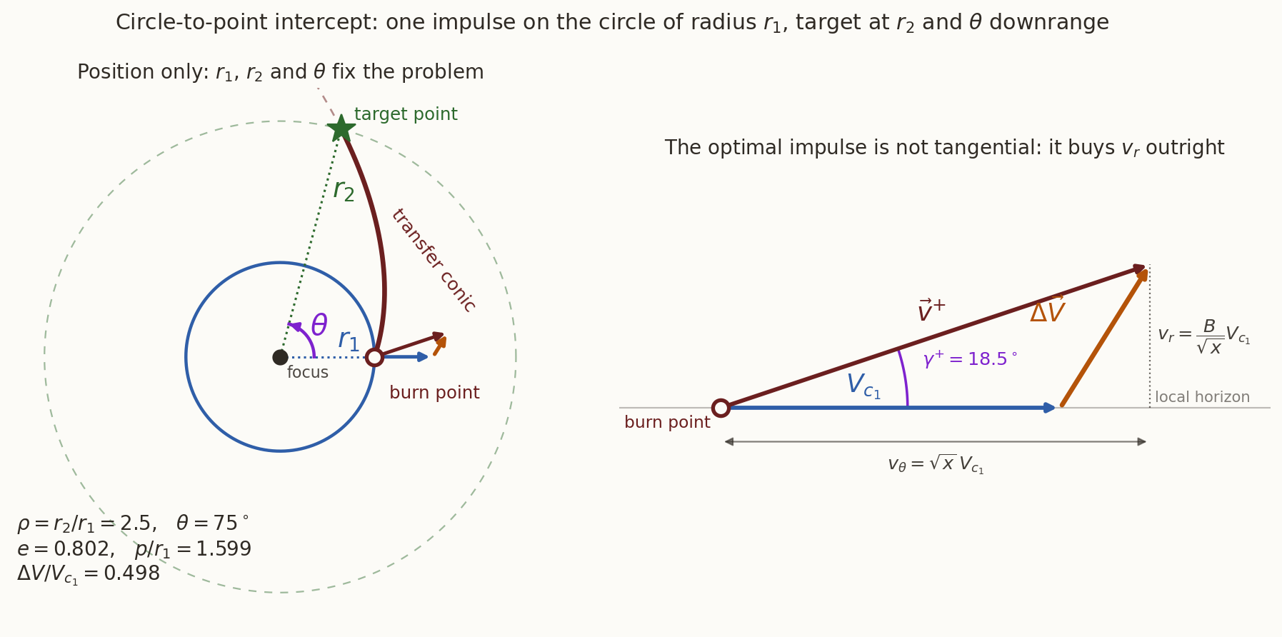
Figure 1: Circle-to-point intercept. Left: the problem is fixed by three numbers — the circular radius \(r_1\), the target radius \(r_2\), and the central angle \(\theta\) between the burn point and the target, measured at the focus in the direction of motion. Right: the velocity triangle at the burn point, to scale. The optimal impulse leaves the orbit at a flight path angle \(\gamma^{+}\ne0\) — it is not tangential.
A one-parameter family of transfer conics
Put the focus at the attracting centre, and let \(f_1\) be the true anomaly at the burn point. Passing through both points gives
\[ \frac{p}{r_1}=1+e\cos f_1, \qquad \frac{p}{r_2}=1+e\cos(f_1+\theta), \]
two conditions on three unknowns \((p,e,f_1)\). One free parameter survives: a whole family of conics joins the two points, and we must pick the cheapest.
Take that parameter to be the dimensionless semi-latus rectum \(x=p/r_1\), and write \(A=e\cos f_1\), \(B=e\sin f_1\). Expanding \(\cos(f_1+\theta)\) and eliminating,
\[ \boxed{\ A(x)=x-1, \qquad B(x)=\frac{(1-\cos\theta)+x\left(\cos\theta-\dfrac{1}{\rho}\right)}{\sin\theta}\ } \]
Everything else follows: \(e=\sqrt{A^2+B^2}\), \(f_1=\operatorname{atan2}(B,A)\), \(a=p/(1-e^2)\).
What the impulse must buy
Before the burn the velocity is purely transverse, of magnitude \(V_{c_1}\). After it,
\[ v_r=\sqrt{\frac{\mu}{p}}\,B, \qquad v_\theta=\frac{\sqrt{\mu p}}{r_1}, \]
so the impulse supplies the radial component outright and makes up the difference in the transverse one:
\[ \boxed{\ J(x)\equiv\left(\frac{\Delta V}{V_{c_1}}\right)^{2} =\underbrace{\frac{B(x)^{2}}{x}}_{\text{radial}} +\underbrace{\left(\sqrt{x}-1\right)^{2}}_{\text{transverse}}\ } \]
- The transverse term is the speed change that alters the angular momentum away from its circular value.
- The radial term is the out-of-tangent component — pure waste in the Oberth sense, and zero only when \(B=0\), i.e. when the burn is tangential.
The quartic
Write \(B=(\beta+\alpha x)/\sin\theta\) with \(\alpha=\cos\theta-1/\rho\) and \(\beta=1-\cos\theta\). Then
\[ \frac{dJ}{dx}=\frac{\alpha^{2}x^{2}-\beta^{2}}{x^{2}\sin^{2}\theta}+1-\frac{1}{\sqrt{x}}, \]
and setting this to zero, multiplying by \(x^{2}\) and putting \(s=\sqrt{x}\):
\[ \boxed{\ \left(\alpha^{2}+\sin^{2}\theta\right)s^{4}-\sin^{2}\theta\;s^{3}-\beta^{2}=0, \qquad s=\sqrt{p/r_1}\ } \]
No \(s^{2}\) or \(s^{1}\) term. Take the positive real roots, evaluate \(J\) at each, keep the smallest — no iterative optimiser anywhere.
The optimum is not generally a tangential burn: \(B=0\) only in special cases. Away from those, the best impulse is applied at an angle to the local horizon — which is exactly why a quartic appears instead of a one-line formula.
From the root to the orbit
The quartic gives \(s\); the transfer conic then follows without any further minimisation. In order,
\[ x=s^{2}=\frac{p}{r_1}, \qquad A=x-1, \qquad B=\frac{\beta+\alpha x}{\sin\theta}, \]
\[ \boxed{\ p=x\,r_1, \qquad e=\sqrt{A^{2}+B^{2}}, \qquad f_1=\operatorname{atan2}(B,A)\ } \]
and everything else is then standard:
\[ a=\frac{p}{1-e^{2}}, \qquad f_2=f_1+\theta, \qquad \frac{v_r}{V_{c_1}}=\frac{B}{\sqrt{x}}, \quad \frac{v_\theta}{V_{c_1}}=\sqrt{x}, \quad \tan\gamma^{+}=\frac{B}{x}. \]
\(\operatorname{atan2}\), not \(\arccos\): \(A\) and \(B\) carry the signs of \(e\cos f_1\) and \(e\sin f_1\) separately, and the quadrant of \(f_1\) is what says whether the burn point is before or after periapsis.
The chain, worked once
Take \(\rho=6\), \(\theta=60^\circ\). Then \(\alpha=\cos\theta-1/\rho=1/2-1/6=1/3\) and \(\beta=1-\cos\theta=1/2\), and the chain above gives
| \(s\) | \(x=s^2\) | \(A\) | \(B\) | \(e\) | \(f_1\) | \(a/r_1\) | \(\Delta V/V_{c_1}\) |
|---|---|---|---|---|---|---|---|
| \(1.093192\) | \(1.195069\) | \(0.195069\) | \(1.037332\) | \(1.05551\) | \(79.35^\circ\) | \(-10.473\) | \(0.95347\) |
The single positive real root of the quartic is \(s=1.093192\); the other roots are \(-0.584\) and a complex pair, all discarded.
\(e>1\) here, so the optimal intercept at \(\rho=6\), \(\theta=60^\circ\) is a hyperbola — \(a\) comes out negative, as it must — which is why the \(60^\circ\) curve is drawn in the hyperbolic line style by the time it reaches \(r_2/r_1=6\). The burn leaves the circle at \(\gamma^{+}=40.96^\circ\) to the local horizon: nowhere near tangential.
Is the arc physical?
A root is admissible only if the spacecraft actually flies the arc at positive radius:
\[ 1+e\cos f>0 \qquad\text{for all } f\in[f_1,\ f_1+\theta]. \]
For an ellipse this is automatic. For a hyperbola it fails if the arc would cross an asymptote, so the test binds only when \(e>1\) and the arc sweeps past the apoapsis direction.
Over the range charted here the constraint never actually binds — but the code tests it rather than assuming it.
\(\theta=180^\circ\): Hohmann falls out
With \(\cos\theta=-1\) we get \(\beta=2\), \(\alpha=-(1+1/\rho)\), and the quartic collapses to \(\alpha^{2}s^{4}=\beta^{2}\):
\[ x=\frac{2\rho}{1+\rho} \qquad\Longleftrightarrow\qquad p=\frac{2r_1r_2}{r_1+r_2}, \]
the semi-latus rectum of the Hohmann ellipse. Here \(\beta+\alpha x=0\), so \(B=0\) and the burn is tangential, as it must be:
\[ \boxed{\ \left.\frac{\Delta V}{V_{c_1}}\right|_{180^\circ} =\left|\sqrt{\frac{2\rho}{1+\rho}}-1\right| \ \longrightarrow\ \sqrt2-1=0.4142\ } \]
This is the lowest curve at every radius ratio: \(180^\circ\) is the cheapest central angle there is.
\(\theta=0\): the rectilinear limit
A conic crosses a ray from the focus exactly once, so no ordinary conic joins two different radii at the same central angle. The optimum degenerates to \(p\to0\): kill the transverse velocity and coast radially.
Setting \(x=k\theta^{2}\) and letting \(\theta\to0\) gives \(v_\theta\to0\) and \(v_r/V_{c_1}\to\sqrt{2(1-1/\rho)}\) — just the energy statement \(v_r^{2}=2\mu(1/r_1-1/r_2)\). Hence
\[ \boxed{\ \left.\frac{\Delta V}{V_{c_1}}\right|_{0} =\begin{cases} 1, & \rho\le 1 \quad(\text{kill } V_{c_1} \text{ and fall}),\\[4pt] \sqrt{3-\dfrac{2}{\rho}}, & \rho>1, \end{cases} \ \longrightarrow\ \sqrt3=1.732\ } \]
The most expensive central angle, and the top curve on the chart. A rectilinear orbit is still a bound conic, which is why it is drawn solid with the ellipses.
The result
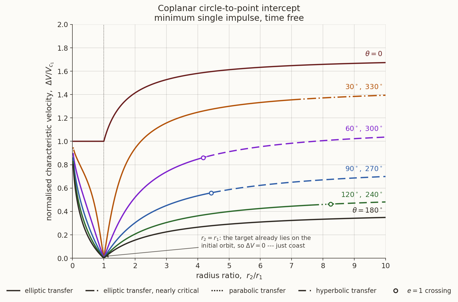
Figure 2: Minimum single-impulse cost to intercept a point at radius \(r_2\), central angle \(\theta\) downrange, from a circular orbit of radius \(r_1\). Line style gives the type of the optimal conic; colour merely separates the central angles. Open circles mark where the optimum passes through \(e=1\). The thumbnails show the geometry behind five of the curves at the marked radius ratio — \(\rho=6\) for \(\theta=0\) to \(90^\circ\), \(\rho=8\) for \(120^\circ\): the circular orbit of radius \(r_1\), the target at \(\rho r_1\) and central angle \(\theta\), and the optimal arc between them, legs to scale. Each is rotated so that its burn-to-target chord lies horizontal.
Reading the chart
Curves come in pairs. Replacing \(\theta\to360^\circ-\theta\) flips the sign of \(\sin\theta\), hence of \(B\) — and \(J\) depends on \(B^{2}\) only. So \(\theta\) and \(360^\circ-\theta\) cost exactly the same: hence the labels \(30^\circ/330^\circ\), \(60^\circ/300^\circ\), and so on.
Everything pinches at \(\rho=1\). The target already lies on the initial orbit, so with time open the answer is to do nothing and coast. Algebraically \(s=1\) solves the quartic identically, giving \(e=0\) and \(J=0\).
Inward (\(\rho<1\)) every curve climbs toward \(\Delta V/V_{c_1}=1\): reaching the centre means destroying essentially all the angular momentum. This branch is the disorbit problem.
Outward (\(\rho>1\)) the curves fan out, monotone in \(\theta\): more central angle is always cheaper, because it lets the burn sit closer to tangential.
When does the ellipse give out?
Small \(\theta\) with large \(\rho\) demands a lot of radius for very little angular travel, which forces high energy. The optimal conic therefore stops being an ellipse beyond a critical radius ratio \(\rho^{*}(\theta)\):
| \(\theta\) | \(20^\circ\) | \(30^\circ\) | \(60^\circ\) | \(70^\circ\) | \(90^\circ\) | \(120^\circ\) | \(150^\circ\) | \(180^\circ\) |
|---|---|---|---|---|---|---|---|---|
| \(\rho^{*}\) | \(50.9\) | \(19.7\) | \(4.19\) | \(\mathbf{3.85}\) | \(4.43\) | \(8.25\) | \(30.1\) | never |
\(\rho^{*}\) is not monotone in \(\theta\). It bottoms out near \(\theta\approx70^\circ\) and climbs steeply at both ends, so the transfers most likely to be non-elliptic are the ones with a moderate central angle — not the smallest. The \(180^\circ\) arc is elliptic for every radius ratio, and the \(30^\circ\) arc stays elliptic across the whole chart but with \(e\to0.99\) — the survey’s “elliptic transfer, nearly critical”.
The code
def intercept(rho, theta):
    """Minimum-dV single-impulse intercept from a circle to a point."""
    c, s = np.cos(theta), np.sin(theta)

    if abs(s) < 1e-12:                              # sin(theta) = 0
        if c > 0:                                   # theta = 0: rectilinear
            dv = 1.0 if rho <= 1.0 else np.sqrt(3.0 - 2.0/rho)
            return dv, np.nan, np.nan, True
        x = 2.0*rho/(1.0 + rho)                     # theta = 180: Hohmann
        return abs(np.sqrt(x) - 1.0), x, abs(x - 1.0), True

    alpha, beta = c - 1.0/rho, 1.0 - c
    roots = np.roots([alpha**2 + s**2, -s**2, 0.0, 0.0, -beta**2])

    best = (np.inf, np.nan, np.nan, True)
    for rt in roots:
        if abs(rt.imag) > 1e-9 or rt.real <= 0.0:
            continue
        x = rt.real**2
        A, B = x - 1.0, (beta + alpha*x)/s           # e cos f1, e sin f1
        J = B*B/x + (np.sqrt(x) - 1.0)**2
        if J >= best[0]:
            continue
        ecc, f1 = np.hypot(A, B), np.arctan2(B, A)
        ff = np.linspace(f1, f1 + theta, 721)
        valid = bool(np.all(1.0 + ecc*np.cos(ff) > 1e-9))
        best = (J, x, ecc, valid)
    return np.sqrt(best[0]), best[1], best[2], best[3]
Full script: codes/fig-man-intercept.py.
Does it work?
The script checks itself against every case with a closed form:
| case | computed | closed form |
|---|---|---|
| \(\theta=180^\circ\), \(\rho=0.5\) | \(0.183503\) | \(0.183503\) |
| \(\theta=180^\circ\), \(\rho=2\) | \(0.154701\) | \(0.154701\) |
| \(\theta=180^\circ\), \(\rho=10\) | \(0.348400\) | \(0.348400\) |
| \(\theta=0\), \(\rho=0.5\) | \(1.000000\) | \(1.000000\) |
| \(\theta=0\), \(\rho=3\) | \(1.527525\) | \(1.527525\) |
| \(\rho=1\), any \(\theta\) | \(\sim10^{-15}\) | \(0\) (coast) |
The quartic roots were also cross-checked against a brute-force dense scan of \(J(x)\) with Brent refinement; the two agree to every printed digit at all \((\rho,\theta)\) tested.
Sample values, \(\Delta V/V_{c_1}\)
| \(\theta\) | \(\rho=0.2\) | \(0.5\) | \(1\) | \(2\) | \(4\) | \(6\) | \(8\) | \(10\) |
|---|---|---|---|---|---|---|---|---|
| \(0\) | \(1.000\) | \(1.000\) | \(1.000\) | \(1.414\) | \(1.581\) | \(1.633\) | \(1.658\) | \(1.673\) |
| \(30^\circ\) | \(0.818\) | \(0.639\) | \(0\) | \(0.940\) | \(1.249\) | \(1.332\) | \(1.371\) | \(1.394\) |
| \(60^\circ\) | \(0.664\) | \(0.405\) | \(0\) | \(0.521\) | \(0.847\) | \(0.953\) | \(1.005\) | \(1.036\) |
| \(90^\circ\) | \(0.550\) | \(0.284\) | \(0\) | \(0.303\) | \(0.534\) | \(0.623\) | \(0.670\) | \(0.699\) |
| \(120^\circ\) | \(0.476\) | \(0.222\) | \(0\) | \(0.207\) | \(0.362\) | \(0.425\) | \(0.459\) | \(0.481\) |
| \(180^\circ\) | \(0.423\) | \(0.184\) | \(0\) | \(0.155\) | \(0.265\) | \(0.309\) | \(0.333\) | \(0.348\) |
The \(\theta=0\) row does not vanish at \(\rho=1\). That discontinuity is real but harmless: \(\theta=0\) admits no ordinary conic, so its curve is the rectilinear limit rather than a member of the same family.
Two caveats from the survey
Minimum \(\Delta V\) \(\ne\) minimum energy. The two coincide only at a \(180^\circ\) central angle. For smaller angles they differ, and taking the minimum-energy path can cost a great deal of extra \(\Delta V\).
If \(\theta>180^\circ\), wait. The \(180^\circ\) solution can always be recovered by coasting on the initial circular orbit until the geometry comes right. So whenever an initial coast is allowed, the upper half of the curve family is of academic interest only — the cheapest practical answer is essentially always the Hohmann-like \(180^\circ\) arc.
Part II — Disorbit to a Prescribed Entry
The problem
Now the target is not a point but an entry interface: reach radius \(r_2<r_1\) with a prescribed entry flight path angle \(\gamma_2\) (negative, descending). The central angle is left open — we do not care where around the globe we come down.
This is the most-studied intercept problem in the whole survey, because it is the re-entry problem.
Work in units of \(V_{c_1}\) and write the post-burn state at \(r_1\) as
\[ w=\frac{v_r}{V_{c_1}}\ (\le 0), \qquad u=\frac{v_\theta}{V_{c_1}} . \]
The pre-burn state is \((0,1)\), so the cost is simply
\[ \left(\frac{\Delta V}{V_{c_1}}\right)^{2}=w^{2}+(u-1)^{2}. \]
The problem, drawn
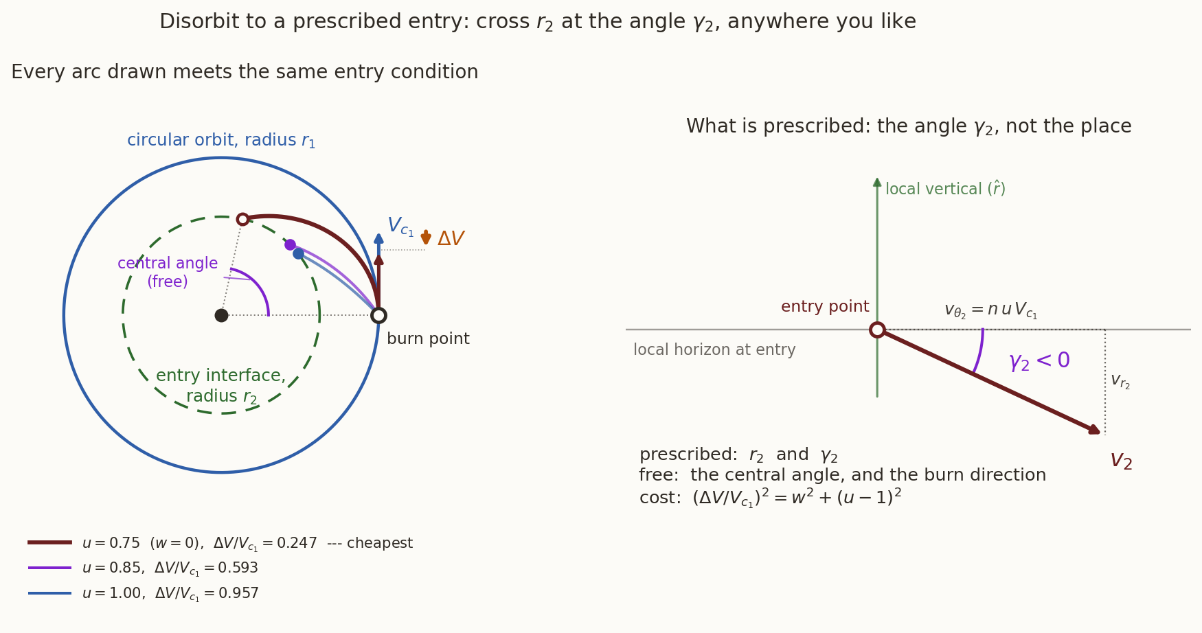
Figure 3: Disorbit to a prescribed entry. Left: three deorbit arcs from the same circular orbit, every one of which crosses the entry radius \(r_2\) at the same flight path angle \(\gamma_2\) — they differ only in the post-burn transverse speed \(u\), and they arrive at quite different central angles, which is precisely what is left free. The cheapest is the horizontal retro burn (\(w=0\)). Right: the entry condition itself — what is prescribed is the angle between \(\vec v_2\) and the local horizon, not where around the globe the crossing happens. Drawn at \(\gamma_2=-25^\circ\) and \(r_1/r_2=1.6\); a real entry corridor is far shallower.
One constraint, one free parameter
Let \(n=r_1/r_2\ge1\). Energy and angular momentum carried to \(r_2\) give
\[ v_2^{2}=V_{c_1}^{2}\left(u^{2}+w^{2}-2+2n\right), \qquad v_{\theta_2}=n\,u\,V_{c_1}, \]
and imposing \(\cos\gamma_2=v_{\theta_2}/v_2\) collapses to a single relation:
\[ \boxed{\ w^{2}=K\,u^{2}-M, \qquad K=\frac{n^{2}}{\cos^{2}\gamma_2}-1, \qquad M=2(n-1)\ } \]
So the cost is a parabola in one variable:
\[ J(u)=(K+1)\,u^{2}-2u+1-M, \qquad \frac{dJ}{du}=0 \;\Longrightarrow\; u=\frac{1}{K+1}. \]
No quartic this time — but there is a catch.
Two regimes
The parabola’s vertex is only usable if the state is physical: \(w^{2}\ge0\) requires \(u\ge\sqrt{M/K}\).
Interior optimum — if \(\dfrac{1}{K+1}\ge\sqrt{\dfrac{M}{K}}\), the vertex is feasible, \(w\ne0\), and the impulse is tilted below the horizon.
Constrained optimum — otherwise the bound bites, the optimum sits on \(w=0\), and the impulse is exactly horizontal with \(u=\sqrt{M/K}\).
The optimal thrust angle below the local horizontal is
\[ \phi=\operatorname{atan2}\!\left(w,\;1-u\right), \]
zero in the second regime. The switch between regimes is the whole story of the figure.
The result
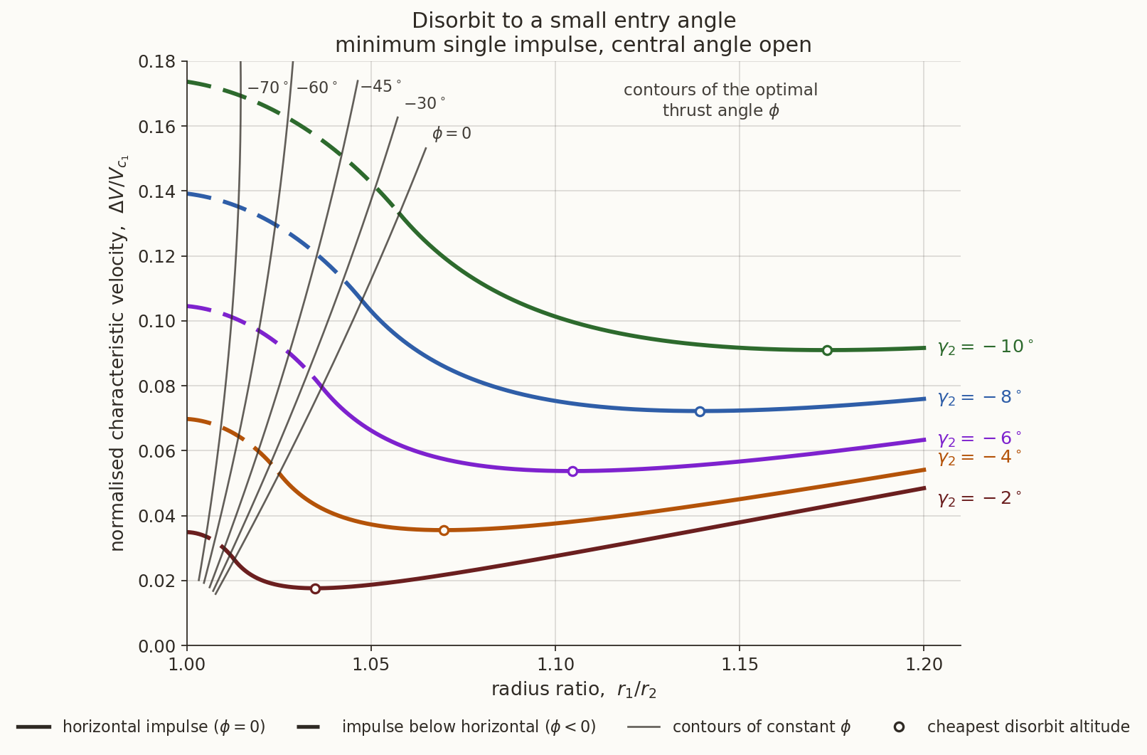
Figure 4: Minimum single-impulse disorbit from a circular orbit of radius \(r_1\) to entry radius \(r_2\) at prescribed entry angle \(\gamma_2\), central angle open. Dashed where the optimal impulse is tilted below the horizon, solid where it is exactly horizontal; thin lines are contours of the optimal thrust angle \(\phi\). Open circles mark the cheapest disorbit altitude on each curve.
Reading the chart
Left edge, \(r_1/r_2=1\). Entry radius equals orbit radius: nothing to do but rotate the velocity vector down through \(\gamma_2\). The impulse is nearly vertical (\(\phi=-(90^\circ-|\gamma_2|)\)) and the cost is at its worst.
Middle. Each curve falls to a minimum — the cheapest disorbit altitude — then climbs again. Deorbiting from too low costs a big rotation; from too high costs a big retro burn.
Right. Every curve is solid: the impulse is purely horizontal, the familiar retro-burn-at-apoapsis picture.
The dashed-to-solid switch on each curve happens well to the left of its minimum, so the cheapest disorbit is always a horizontal retro burn. The tilted-impulse regime is real but never optimal once you are free to choose the altitude.
Closed forms that fall out
The chart is usually quoted graphically, but both regimes integrate in closed form.
At \(r_1=r_2\) the whole manoeuvre is a velocity rotation, and
\[ \boxed{\ \left.\frac{\Delta V}{V_{c_1}}\right|_{n=1}=\left|\sin\gamma_2\right|\ } \]
In the horizontal regime (\(w=0\)),
\[ \boxed{\ \frac{\Delta V}{V_{c_1}}=1-\cos\gamma_2\sqrt{\frac{2(n-1)}{n^{2}-\cos^{2}\gamma_2}}\ } \]
Maximising that square root gives \(n^{2}-2n+\cos^{2}\gamma_2=0\), so the cheapest disorbit altitude and its cost are
\[ \boxed{\ \left(\frac{r_1}{r_2}\right)_{\rm best}=1+\left|\sin\gamma_2\right|, \qquad \frac{\Delta V_{\min}}{V_{c_1}}=1-\frac{\cos\gamma_2}{\sqrt{1+\left|\sin\gamma_2\right|}}\ } \]
Checking the closed forms
| \(\gamma_2\) | \(\left|\sin\gamma_2\right|\) | \(\Delta V\) at \(n=1\) | best \(r_1/r_2\) | \(\Delta V_{\min}\) |
|---|---|---|---|---|
| \(-2^\circ\) | \(0.034899\) | \(0.034899\) | \(1.0349\) | \(0.01761\) |
| \(-4^\circ\) | \(0.069756\) | \(0.069756\) | \(1.0698\) | \(0.03551\) |
| \(-6^\circ\) | \(0.104528\) | \(0.104528\) | \(1.1045\) | \(0.05371\) |
| \(-8^\circ\) | \(0.139173\) | \(0.139173\) | \(1.1392\) | \(0.07219\) |
| \(-10^\circ\) | \(0.173648\) | \(0.173648\) | \(1.1737\) | \(0.09096\) |
Columns 2 and 3 agree to every digit, and the “best \(r_1/r_2\)” column is exactly \(1+\left|\sin\gamma_2\right|\) — so the numerical optimiser and the closed forms are the same answer.
The \(1.125\) rule
The survey states (p. 11) that
If \(r_1/r_2>1.125\) the impulse is always horizontal, and it is below horizontal for \(r_1/r_2<1.125\).
That constant is the maximum over all entry angles of the regime boundary \(\frac{1}{K+1}=\sqrt{M/K}\). Solving it here gives
\[ \boxed{\ \left(\frac{r_1}{r_2}\right)_{\max}=1.1250 \quad\text{attained at}\quad \gamma_2\approx-37.3^\circ\ } \]
The boundary is not monotone in \(\gamma_2\): it rises from \(1\) at \(\gamma_2=0\), peaks at \(1.125\) near \(-37^\circ\), and falls back toward \(1\) as \(\gamma_2\to-90^\circ\). The report quotes only the peak — reconstructing the curve shows where the peak comes from, and that the shallow entry angles of practical interest switch over much earlier (at \(r_1/r_2\approx1.013\) for \(-2^\circ\), \(1.058\) for \(-10^\circ\)).
Part III — Escape from a Circular Orbit
Specified energy
Now nothing about where is prescribed — only how much energy. Leave the circular orbit of radius \(r_1\) on a hyperbola with a given hyperbolic excess speed \(V_\infty\); the pericentre distance and the axis orientation are free.
To have excess speed \(V_\infty\) after coasting out from radius \(r\),
\[ v^{2}=V_\infty^{2}+\frac{2\mu}{r}, \]
so with \(x=V_\infty/V_{c_1}\) and \(V_{\rm esc}=\sqrt2\,V_{c_1}\) at \(r_1\), a single tangential impulse costs
\[ \boxed{\ \frac{\Delta V_1}{V_{c_1}}=\sqrt{x^{2}+2}-1\ } \]
But there is no rule that says you must burn at \(r_1\) — and the \(2\mu/r\) makes burning deeper more productive. That is the whole idea.
Three ways out
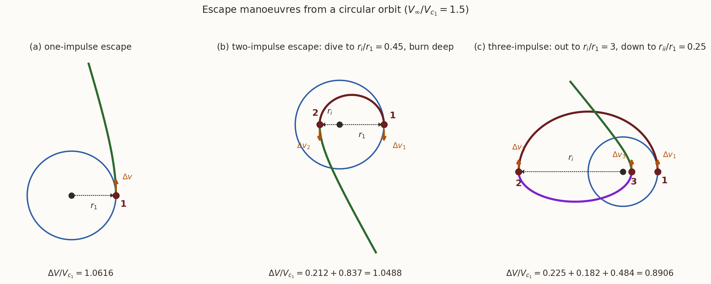
Figure 5: The same escape (\(V_\infty/V_{c_1}=1.5\)) flown three ways, drawn as true conics. (a) burn once on the circle; (b) drop to \(r_i\) and burn deep, where the Oberth benefit is larger; (c) coast out to \(r_i\), drop the pericentre to \(r_{ii}\) almost for free, then escape from very deep. Costs are per-panel totals.
What the three modes cost
With \(k=r_i/r_1\), the two-impulse dive costs
\[ \frac{\Delta V_2}{V_{c_1}} =\underbrace{1-\sqrt{\frac{2k}{1+k}}}_{\text{drop to } r_i} +\underbrace{\sqrt{x^{2}+\frac{2}{k}}-\sqrt{\frac{2}{k(1+k)}}}_{\text{escape from } r_i} \]
For the case drawn (\(x=1.5\)):
| mode | \(\Delta V/V_{c_1}\) |
|---|---|
| (a) one impulse | \(1.0616\) |
| (b) two impulses, \(r_i/r_1=0.45\) | \(1.0488\) |
| (c) three impulses, \(r_i/r_1=3\), \(r_{ii}/r_1=0.25\) | \(\mathbf{0.8906}\) |
When does diving pay?
Set \(x=\sqrt2\), i.e. \(V_\infty=V_{\rm esc}\). The second bracket becomes
\[ \sqrt{\frac{2}{k}}\left(\sqrt{1+k}-\frac{1}{\sqrt{1+k}}\right) =\sqrt{\frac{2}{k}}\cdot\frac{k}{\sqrt{1+k}} =\sqrt{\frac{2k}{1+k}}, \]
which exactly cancels the first bracket. So
\[ \boxed{\ V_\infty=V_{\rm esc}\ \Longrightarrow\ \frac{\Delta V_1}{V_{c_1}}=\frac{\Delta V_2}{V_{c_1}}=1 \quad\text{for \textit{every} } r_i\ } \]
\(V_\infty=V_{\rm esc}\) is a watershed, and \(r_i\) drops out of the arithmetic entirely there. Below it the single impulse wins; above it the dive always wins, by more the faster you need to leave. Verified numerically: the two-impulse cost is \(1.0000000000\) for \(r_i/r_1 = 0.9,\,0.5,\,0.1,\,0.01\) alike.
The whole trade, in one chart
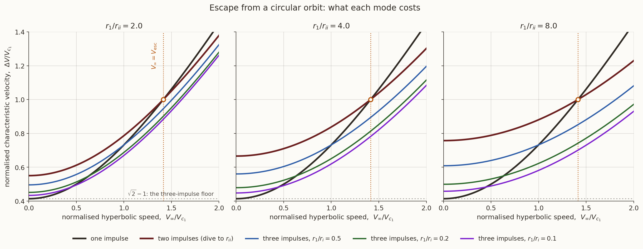
Figure 6: Cost of each escape mode against the hyperbolic excess speed. Each panel fixes the depth \(r_1/r_{ii}\); all curves in a panel dive to the same \(r_{ii}\), so the comparison is at equal depth. The dotted vertical is \(V_\infty=V_{\rm esc}\); the ringed point is where the one- and two-impulse curves cross.
Reading the chart
The crossing is fixed. In every panel the one-impulse (black) and two-impulse (maroon) curves meet at exactly \((\sqrt2,\,1)\) — the identity of the previous slide, now visible. Left of it the single burn wins; right of it the dive does.
Depth is a double-edged tool. Going deeper (moving right across the panels) raises the two-impulse curve at low \(V_\infty\) but lowers it at high \(V_\infty\). At \(V_\infty/V_{c_1}=2\) and \(r_1/r_{ii}=8\), two impulses cost \(1.230\) against the single burn’s \(1.450\).
Three impulses dominate at speed. The gain grows with both \(V_\infty\) and \(r_i\): at \(r_1/r_{ii}=8\), \(V_\infty/V_{c_1}=2\), going out to \(r_i=10r_1\) first costs \(0.931\) — a \(36\%\) saving on the single impulse.
At small \(V_\infty\) every multi-impulse curve sits above the single burn. There is nothing to gain from cleverness when you barely need to escape.
The cancellation is general
At \(V_\infty=V_{\rm esc}(r_1)\) the dive depth dropped out. That was not special to \(r_1\) — the same thing happens one level up:
\[ \boxed{\ V_\infty=V_{\rm esc}(R)=\sqrt{\frac{2\mu}{R}} \ \Longrightarrow\ \text{the depth of a dive begun at } R \text{ does not matter}\ } \]
Applied at the intermediate apoapsis \(r_i\), burns 2 and 3 of the three-impulse mode become independent of \(r_{ii}\) exactly when \(V_\infty=\sqrt{2\mu/r_i}\):
| \(r_i/r_1\) | \(V_\infty/V_{c_1}\) | spread over \(r_{ii}/r_1\in[0.02,\,0.5]\) |
|---|---|---|
| \(2\) | \(0.700\) (below) | \(9.2\times10^{-2}\) |
| \(2\) | \(\mathbf{1.000}\) (at) | \(\mathbf{1.4\times10^{-15}}\) |
| \(2\) | \(1.300\) (above) | \(1.2\times10^{-1}\) |
| \(5\) | \(\mathbf{0.632}\) (at) | \(\mathbf{5.6\times10^{-16}}\) |
| \(10\) | \(\mathbf{0.447}\) (at) | \(\mathbf{4.4\times10^{-16}}\) |
Below that speed diving deeper hurts; above it, diving deeper helps. The report notes the special case at \(r_1\); the general rule explains why the chart looks the way it does.
The limit: escape for the price of a parabola
Push the three-impulse mode to its extreme — \(r_i/r_1\to\infty\) (parabolic intermediate arcs) and \(r_{ii}/r_1\to0\) (grazing the focus). The first burn tends to the parabolic escape burn, and the other two tend to zero:
\[ \boxed{\ \frac{\Delta V_3}{V_{c_1}}\longrightarrow\sqrt2-1=0.4142 \quad\text{for \textit{any} } V_\infty\ } \]
| \(V_\infty/V_{c_1}\) | \(r_i/r_1=10^3\) | \(10^6\) | \(10^9\) |
|---|---|---|---|
| \(1.5\) | \(0.4400\) | \(0.4150\) | \(0.4142\) |
| \(3.0\) | \(0.5154\) | \(0.4174\) | \(0.4143\) |
| \(6.0\) | \(0.8156\) | \(0.4269\) | \(0.4146\) |
Any hyperbolic excess speed, for the cost of barely escaping — paid for with unbounded flight time and a pass through the centre of the planet. The survey’s own caveat is the practical one: if the manoeuvre is constrained to the space outside the circular orbit, a single impulse is always the optimum coplanar escape mode. Every saving here comes from diving inside \(r_1\).
Part IV — Transfer: the Hohmann Summary
One chart for the whole problem
The survey closes its transfer section with a single picture: the circle-to-circle Hohmann transfer over four decades of radius ratio. With \(R=r_2/r_1\) and \(V_{c_1}=\sqrt{\mu/r_1}\),
\[ \frac{\Delta v_1}{V_{c_1}}=\left|\sqrt{\frac{2R}{1+R}}-1\right|, \qquad \frac{\Delta v_2}{V_{c_1}}=\left|\frac{1}{\sqrt R}-\sqrt{\frac{2}{R(1+R)}}\right| . \]
The absolute values do real work: they let one chart carry both directions. \(R>1\) is the climb, \(R<1\) the descent, and by the time-reversal symmetry of Part I of the Orbital Maneuvers deck the magnitudes are the same either way — only the sense of each burn flips.
Nothing here is new physics — the derivation is in the other deck. What is new is the range: plotting it from \(R=0.01\) to \(R=100\) shows behaviour that a LEO-to-GEO example cannot.
The chart
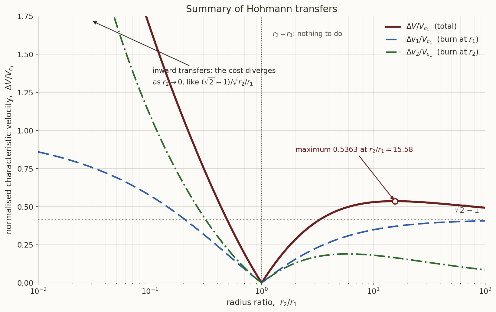
Figure 7: Hohmann transfer between coplanar circles: the total and the two burns separately, normalised by \(V_{c_1}\), over four decades of radius ratio. The dotted horizontal is the outward asymptote \(\sqrt2-1\); the ringed point is the non-monotone maximum.
What four decades show
Outward, the cost is not monotone. It climbs to \(\Delta V/V_{c_1}=0.5363\) at \(R=15.58\), then falls toward \(\sqrt2-1=0.4142\). Going further can cost less — the seed of the bi-elliptic transfer, and the same \(15.58\) that governs it.
The split changes character. \(\Delta v_1\) rises monotonically to \(\sqrt2-1\) (the departure burn becomes an escape burn), while \(\Delta v_2\) peaks near \(R\approx5.9\) and then decays to zero — arriving somewhere very far away is nearly free, because you get there barely moving.
Inward, there is no asymptote. As \(r_2\to0\) the cost diverges like \((\sqrt2-1)/\sqrt{r_2/r_1}\): at \(R=0.01\) the total is \(4.93\,V_{c_1}\), right off the top of the frame. Only \(\Delta v_1\) stays bounded, tending to \(1\) — you can never spend more than the whole circular velocity on the first burn.
Tying the decks together
Evaluating the same two formulas at LEO and GEO (\(r_1=6678.137\) km, \(r_2=42164\) km, so \(R=6.31374\), \(V_{c_1}=7.72576\) km/s):
\[ \boxed{\ \Delta v_1=2.42573,\quad \Delta v_2=1.46682,\quad \Delta V=3.89255\ \mathrm{km/s}\ } \]
which is Example 1 of the Orbital Maneuvers deck, to all five decimals.
Two independent routes — a worked numerical example there, a normalised universal chart here — meeting on the same number. That agreement is the point of normalising by \(V_{c_1}\) in the first place: one curve serves every central body and every pair of radii.
What to remember
Intercept (Part I)
- Intercept matches position only, so it costs one impulse, not two.
- The transfer conics through two points form a one-parameter family; minimising over it gives a quartic in \(\sqrt{p/r_1}\), not a formula.
- The optimal burn is generally not tangential. Tangency is recovered only in the degenerate cases.
- \(\theta\) and \(360^\circ-\theta\) cost the same; \(180^\circ\) is always cheapest and reproduces Hohmann; \(\theta=0\) is always dearest and is the rectilinear limit.
- Optimal arcs go non-elliptic first at moderate central angles (\(\rho^{*}\) minimal near \(70^\circ\)), not at the smallest ones.
Disorbit (Part II)
- Matching an entry angle as well as an entry radius leaves one free variable and a parabola, not a quartic — but with an inequality constraint that does the interesting work.
- The constraint is \(w^2\ge0\): when it bites, the optimal impulse is exactly horizontal. That is the ordinary retro burn, and it is always the regime containing the cheapest disorbit altitude.
- Best altitude and cost in closed form: \(r_1/r_2=1+\left|\sin\gamma_2\right|\) and \(\Delta V_{\min}/V_{c_1}=1-\cos\gamma_2/\sqrt{1+\left|\sin\gamma_2\right|}\).
Escape (Part III)
- One impulse costs \(\sqrt{x^{2}+2}-1\) with \(x=V_\infty/V_{c_1}\); burning deeper beats it once \(V_\infty>V_{\rm esc}\), and ties it exactly at \(V_\infty=V_{\rm esc}\) for any dive depth. More generally, a dive begun at radius \(R\) is depth-indifferent precisely when \(V_\infty=V_{\rm esc}(R)\).
- Three impulses beat both, and in the limit deliver any \(V_\infty\) for \(\sqrt2-1\) — but only by going inside \(r_1\). Forbid that and one impulse is optimal again.
Transfer (Part IV)
- Over four decades the Hohmann cost is non-monotone outward (max \(0.5363\) at \(R=15.58\), then down to \(\sqrt2-1\)) and unbounded inward (like \(1/\sqrt R\)). Descending to a small radius is the expensive direction, not ascending.
Source
F. W. Gobetz and J. R. Doll, A Survey of Impulsive Trajectories, United Aircraft Research Laboratories Report G-910557-11, Contract NAS8-21091, Final Report, June 1968. Figures 1–5 (pp. 77–81); discussion pp. 9–22.
Local copy: references/nasa-report-orbit-maneuvers.pdf in the notes repository. Both charts here are reconstructions from the equations above, not scans — which is what let us add the \(e=1\) crossings, the \(\rho^{*}\) table, the closed forms for the best disorbit altitude, an independent check of the \(1.125\) constant, and the \(\sqrt2-1\) escape limit.
Scripts: codes/fig-man-intercept-geom.py, codes/fig-man-intercept.py, codes/fig-man-disorbit-geom.py, codes/fig-man-disorbit.py, codes/fig-man-escape.py, codes/fig-man-escape-cost.py, codes/fig-man-hohmann-summary.py.

SFM, IIST 2026