Perifocal Coordinate System

From the conic in its own plane to the inertial state vector

Devendra Ghate

Where this deck sits

The classical time-of-flight equations for the three conic types are already in hand.

For elliptic motion,

\[ M = E - e\sin E . \]

For parabolic motion, Barker’s equation gives the time relation. For hyperbolic motion,

\[ M_h = e\sinh H - H . \]

All three answer the same physical question:

Given the elapsed time, where is the body along the conic?

But none of them yet produces a state vector. They give a scalar position along a curve; flight software, tracking and manoeuvre design all need \((\mathbf r,\mathbf v)\) in an inertial frame.

Two questions, two routes

1. Once the location on the conic is known, how do we express position and velocity as vectors?
2. Can we propagate the Cartesian state directly, without changing the formulation between elliptic, parabolic and hyperbolic motion?

The first question leads to the perifocal frame — this deck. The second leads to the Lagrange \(f\) and \(g\) functions, and then to the universal-variable formulation.

\[ \text{classical, element-based:}\qquad \Delta t \;\rightarrow\; E,\ D,\ H \;\rightarrow\; f \;\rightarrow\; \mathbf r_{PQW},\mathbf v_{PQW} \;\rightarrow\; \mathbf r_I,\mathbf v_I . \]

\[ \text{universal, state-vector:}\qquad \Delta t \;\rightarrow\; \chi \;\rightarrow\; f,g,\dot f,\dot g \;\rightarrow\; \mathbf r,\mathbf v . \]

The two routes are not rivals. The classical one is transparent and is what orbital elements are for; the universal one is what you implement when the code must not branch on conic type.

The perifocal frame

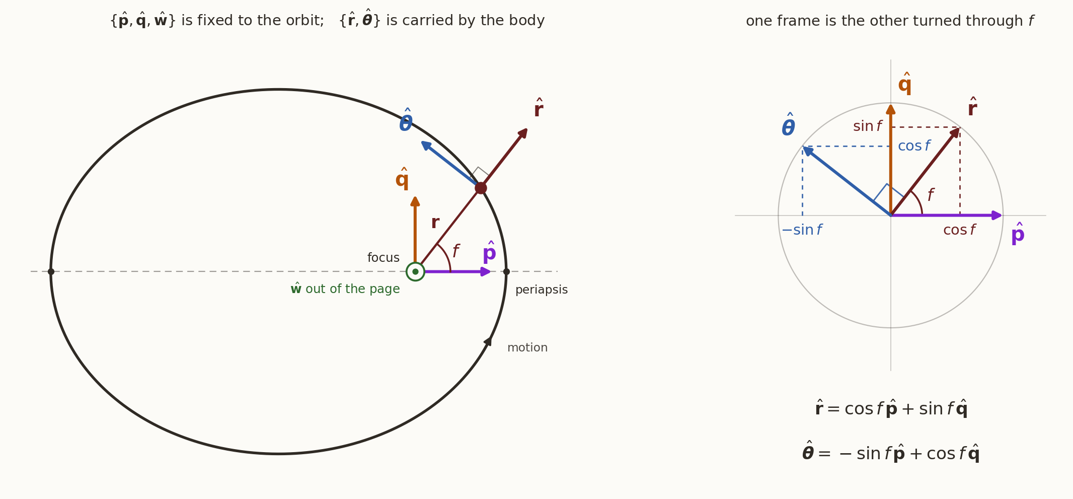
Figure 1: Left: the conic in its own plane. The perifocal basis \(\{\hat{\mathbf p},\hat{\mathbf q},\hat{\mathbf w}\}\) is pinned to the orbit — \(\hat{\mathbf p}\) from the focus to periapsis, \(\hat{\mathbf q}\) a right angle ahead of it in the direction of motion, \(\hat{\mathbf w}=\mathbf h/h\) out of the plane — so it never turns. The polar basis \(\{\hat{\mathbf r},\hat{\boldsymbol\theta}\}\) is carried by the body, so it turns at the rate \(\dot f\). Right: the only relation between them. Both are orthonormal and both lie in the orbital plane, so one is the other rotated through the true anomaly \(f\). Download the script.

Definition of the frame

Suppose the orbit is known through its geometric parameters \(p\), \(e\) and \(f\). The polar equation of the conic,

\[ r = \frac{p}{1+e\cos f}, \]

gives the scalar distance from the focus. To build a vector representation, introduce the perifocal frame \(\{\hat{\mathbf p},\hat{\mathbf q},\hat{\mathbf w}\}\), centred at the active focus:

• \(\hat{\mathbf p}\) points from the focus toward periapsis;
• \(\hat{\mathbf q}\) lies in the orbital plane, \(90^\circ\) ahead of \(\hat{\mathbf p}\) in the direction of motion;
• \(\hat{\mathbf w}\) is normal to the orbital plane.

Since the specific angular momentum is \(\mathbf h=\mathbf r\times\mathbf v\), we define

\[ \hat{\mathbf w}=\frac{\mathbf h}{h}, \qquad\text{so that}\qquad \hat{\mathbf p}\times\hat{\mathbf q}=\hat{\mathbf w} \]

and the triad is right-handed. Both \(\mathbf h\) and the apse line are constants of the two-body motion, so the perifocal frame is fixed in inertial space — it is a genuine inertial frame, not a rotating one, and no fictitious forces arise in it.

Position in the perifocal frame

Because true anomaly is measured from periapsis, i.e. from \(\hat{\mathbf p}\),

\[ \hat{\mathbf r} = \cos f\,\hat{\mathbf p} + \sin f\,\hat{\mathbf q}, \]

which is the right-hand panel of Figure 1. Therefore \(\mathbf r = r\,\hat{\mathbf r}\) gives

\[ \mathbf r = r \left( \cos f\,\hat{\mathbf p} + \sin f\,\hat{\mathbf q} \right), \]

and in components,

\[ \boxed{\; \mathbf r_{PQW} = r \begin{bmatrix} \cos f\\ \sin f\\ 0 \end{bmatrix} = \frac{p}{1+e\cos f} \begin{bmatrix} \cos f\\ \sin f\\ 0 \end{bmatrix}. \;} \]

The third component is identically zero — that is the whole point of the frame. A three-dimensional problem has been reduced to a two-dimensional one, and the missing dimension is restored later by a single rotation.

Velocity: the two terms

Differentiating \(\mathbf r = r\,\hat{\mathbf r}\),

\[ \mathbf v = \dot r\,\hat{\mathbf r} + r\,\dot{\hat{\mathbf r}} = \dot r\,\hat{\mathbf r} + r\dot f\,\hat{\boldsymbol\theta}, \]

using \(\dot{\hat{\mathbf r}}=\dot f\,\hat{\boldsymbol\theta}\): the unit vector \(\hat{\mathbf r}\) cannot change length, only direction, and it turns at the rate \(\dot f\).

Two terms, two meanings:

term	name	vanishes when
\(\dot r\)	radial speed \(v_r\)	at the apsides, \(f=0,\pi\)
\(r\dot f\)	transverse speed \(v_\perp\)	never (for \(h\neq0\))

We now evaluate each in terms of \((p,e,f)\) alone.

The transverse term

From the constancy of angular momentum,

\[ h=r^{2}\dot f \qquad\Longrightarrow\qquad r\dot f=\frac{h}{r}=\frac{\sqrt{\mu p}}{r}, \]

where \(h=\sqrt{\mu p}\). Substituting the conic equation for \(r\),

\[ r\dot f = \sqrt{\mu p}\,\frac{1+e\cos f}{p} = \sqrt{\frac{\mu}{p}}\,(1+e\cos f). \]

The radial term

Differentiating the conic equation with respect to \(f\),

\[ \frac{dr}{df} = \frac{pe\sin f}{(1+e\cos f)^{2}} = \frac{r^{2}e\sin f}{p}, \]

since \(r=p/(1+e\cos f)\) makes \((1+e\cos f)^{-2}=r^{2}/p^{2}\). Then, by the chain rule and \(\dot f = h/r^{2}\),

\[ \dot r = \frac{dr}{df}\,\dot f = \frac{r^{2}e\sin f}{p}\cdot\frac{h}{r^{2}} = \frac{he\sin f}{p} = \sqrt{\frac{\mu}{p}}\;e\sin f . \]

Note that \(r\) cancels completely: both velocity components depend on \(f\) only, never on where the body is. This is the algebraic root of the velocity hodograph being a circle.

Velocity in the polar basis

Collecting the two results,

\[ \boxed{\; \mathbf v = \sqrt{\frac{\mu}{p}} \left[ e\sin f\,\hat{\mathbf r} + (1+e\cos f)\,\hat{\boldsymbol\theta} \right]. \;} \]

This is already a complete answer — but in the rotating basis \(\{\hat{\mathbf r},\hat{\boldsymbol\theta}\}\), which is useless for adding vectors at two different instants. So convert to the fixed basis using

\[ \begin{aligned} \hat{\mathbf r} & = \cos f\,\hat{\mathbf p} + \sin f\,\hat{\mathbf q},\\ \hat{\boldsymbol\theta} & = -\sin f\,\hat{\mathbf p} + \cos f\,\hat{\mathbf q}. \end{aligned} \]

Projecting onto \(\hat{\mathbf p}\) and \(\hat{\mathbf q}\)

\[ \mathbf v = \sqrt{\frac{\mu}{p}} \left[ e\sin f (\cos f\,\hat{\mathbf p}+\sin f\,\hat{\mathbf q}) + (1+e\cos f) (-\sin f\,\hat{\mathbf p}+\cos f\,\hat{\mathbf q}) \right]. \]

The \(\hat{\mathbf p}\) coefficient is

\[ e\sin f\cos f - \sin f - e\sin f\cos f = -\sin f . \]

The \(\hat{\mathbf q}\) coefficient is

\[ e\sin^{2} f + \cos f + e\cos^{2} f = e+\cos f . \]

Both simplifications are pure cancellation — the \(e\sin f\cos f\) terms in the first, the Pythagorean identity in the second.

The perifocal state vector

\[ \boxed{\; \mathbf r_{PQW} = \frac{p}{1+e\cos f} \begin{bmatrix} \cos f\\ \sin f\\ 0 \end{bmatrix}, \qquad \mathbf v_{PQW} = \sqrt{\frac{\mu}{p}} \begin{bmatrix} -\sin f\\ e+\cos f\\ 0 \end{bmatrix}. \;} \]

Since \(h=\sqrt{\mu p}\), the velocity is often written

\[ \mathbf v_{PQW} = \frac{\mu}{h} \begin{bmatrix} -\sin f\\ e+\cos f\\ 0 \end{bmatrix}, \]

which is the form used when \(h\), rather than \(a\), is carried as the size element.

Nothing in this derivation assumed \(e<1\). The pair holds for every conic — ellipse, parabola (\(e=1\), where \(a\) is useless but \(p\) is finite) and hyperbola — because it was built from \(p\), \(e\) and \(f\), never from \(a\).

Two facts you can read off the boxed result

The velocity hodograph is a circle. The velocity components are \(\sqrt{\mu/p}\,(-\sin f,\;e+\cos f)\). As \(f\) runs over the orbit the tip of \(\mathbf v\) traces

\[ v_P^{2}+\left(v_Q-e\sqrt{\tfrac\mu p}\right)^{2}=\frac{\mu}{p}, \]

a circle of radius \(\sqrt{\mu/p}=\mu/h\) centred at \((0,\ e\mu/h)\) — offset, but a circle for every eccentricity.

Periapsis and apoapsis speeds follow by setting \(f=0,\pi\):

\[ v_p=\sqrt{\frac\mu p}\,(1+e), \qquad v_a=\sqrt{\frac\mu p}\,(1-e), \qquad \frac{v_p}{v_a}=\frac{1+e}{1-e}, \]

which is the ratio that drives the Oberth effect and every apsidal manoeuvre.

Why the perifocal frame is useful

The perifocal frame separates two independent pieces of information.

The conic equation describes the geometry within the orbital plane:

\[ r=\frac{p}{1+e\cos f}. \]

The angles \(\Omega\), \(i\), \(\omega\) describe how that plane is oriented in inertial space. Thus

\[ \boxed{ \text{conic geometry} \;+\; \text{orbital orientation} \;=\; \text{inertial state}. } \]

The perifocal frame is the natural bridge between scalar orbital geometry and three-dimensional vectors: everything hard about the dynamics lives on the left, and everything hard about the bookkeeping lives on the right.

Rotation from perifocal to inertial coordinates

Let the inertial frame be \(\{\hat{\mathbf I},\hat{\mathbf J},\hat{\mathbf K}\}\). Both vectors transform with the same matrix, because a rotation acts on vectors, not on their physical meaning:

\[ \mathbf r_I = \mathbf Q_{PQW\rightarrow I}\, \mathbf r_{PQW}, \qquad \mathbf v_I = \mathbf Q_{PQW\rightarrow I}\, \mathbf v_{PQW}. \]

Using the standard orbital-element sequence — the 3–1–3 Euler sequence,

\[ \mathbf Q_{PQW\rightarrow I} = \mathbf R_3(\Omega)\, \mathbf R_1(i)\, \mathbf R_3(\omega). \]

Read right to left, in the order the rotations are applied: \(\omega\) turns \(\hat{\mathbf p}\) back onto the line of nodes, \(i\) lays the orbital plane onto the reference plane, \(\Omega\) swings the node line onto \(\hat{\mathbf I}\).

The elementary rotations

For an active rotation (of the vector, with the frame held still),

\[ \mathbf R_3(\theta) = \begin{bmatrix} \cos\theta & -\sin\theta & 0\\ \sin\theta & \cos\theta & 0\\ 0&0&1 \end{bmatrix}, \qquad \mathbf R_1(\theta) = \begin{bmatrix} 1&0&0\\ 0&\cos\theta&-\sin\theta\\ 0&\sin\theta&\cos\theta \end{bmatrix}. \]

Convention trap

Many texts define \(\mathbf R_3\) as rotating the frame rather than the vector, and so tabulate the transpose of everything below. The two differ by \(\theta\rightarrow-\theta\) throughout. Check one case you know before trusting a formula: \(\Omega=i=\omega=0\) must give \(\mathbf Q=\mathbf 1\).

The direction cosine matrix

\[ \mathbf Q_{PQW\rightarrow I} = \begin{bmatrix} \cos\Omega\cos\omega-\sin\Omega\sin\omega\cos i & -\cos\Omega\sin\omega-\sin\Omega\cos\omega\cos i & \sin\Omega\sin i \\ \sin\Omega\cos\omega+\cos\Omega\sin\omega\cos i & -\sin\Omega\sin\omega+\cos\Omega\cos\omega\cos i & -\cos\Omega\sin i \\ \sin\omega\sin i & \cos\omega\sin i & \cos i \end{bmatrix}. \]

Its three columns are \(\hat{\mathbf p}\), \(\hat{\mathbf q}\), \(\hat{\mathbf w}\) written in inertial components. Two checks:

• the third column carries no \(\omega\) — turning the apse line inside the plane cannot move the plane’s normal;
• the third row carries \(\sin i\) throughout, and vanishes at \(i=0\) — an equatorial orbit has no out-of-plane component.

\(\mathbf Q\) is orthogonal, so the inverse map is free: \(\mathbf r_{PQW}=\mathbf Q^{\mathsf T}\mathbf r_I\).

The classical propagation chain

\[ \boxed{ \Delta t \;\rightarrow\; \text{anomaly } (E,\,D,\,H) \;\rightarrow\; f \;\rightarrow\; \mathbf r_{PQW},\mathbf v_{PQW} \;\rightarrow\; \mathbf r_I,\mathbf v_I . } \]

Each arrow is one idea:

1. \(\Delta t\rightarrow\) anomaly is Kepler’s equation — the only transcendental step.
2. anomaly \(\rightarrow f\) is a half-angle identity.
3. \(f\rightarrow\mathbf r_{PQW},\mathbf v_{PQW}\) is this deck: the conic, in its own plane.
4. \(\mathbf r_{PQW},\mathbf v_{PQW}\rightarrow\mathbf r_I,\mathbf v_I\) is one \(3\times3\) rotation built from \(\Omega\), \(i\), \(\omega\).

Step 3 is where the geometry becomes a vector; step 4 is where the vector acquires an address in the sky.