Problem at Hand
We wish to first explain and then predict the state of each planet in our solar system at any given time.
Lets start with the most naive approach to this problem, which is to consider the planets and the sun as spherical bodies (which is an approximation) and then use Newton’s law of gravitation to compute the forces acting on each body.
This leads to the celebrated N Body Problem in celestial mechanics.
History
Very rich; we will start with Tycho Brahe
- Took very accurate measurements over decades and passed on ( ? ) the data to Kepler
Kepler formulated three laws (1709-1719) using pure data analysis and kinematic assumptions
Kepler’s Laws
- First Law: The orbit of a planet is an ellipse with the Sun at one of the two foci.
- Second Law: A line segment joining a planet and the Sun sweeps out equal areas during equal intervals of time (\(r\cdot\dot{r} = const\)).
- Third Law: The square of the orbital period of a planet is directly proportional to the cube of the semi-major axis of its orbit. (\(T^2 \propto a^3\))
Kepler’s laws were derived from data and not from any physical principles. Newton was the first to provide a physical explanation for Kepler’s laws using his law of gravitation.
Solar System
It is made up of the Sun, planets, moons, asteroids, comets and other small bodies. There are \(n\) bodies.
These are of different sizes and masses, with internally varying density. The Sun is the largest body in the solar system, and it contains more than 99% of the total mass of the solar system.
Since the radius of Sun is \(R_\odot \sim 7 \times 10^8\) m, radius of Earth is \(R_\oplus \sim 6.4 \times 10^6\) m, and the distance between them is \(r \sim 1.5 \times 10^{11}\) m. Therefore, \(R_\odot/r \sim 0.005\) and \(R_\oplus/r \sim 0.00004\). Hence, we can consider the Sun and the Earth as point masses.
Therefore we can consider the bodies as point masses, and use Newton’s law of gravitation to compute the forces acting on each body.
We will give a separate justification for the Earth and the satellite systems later in the course.
Newton’s Law of Gravitation
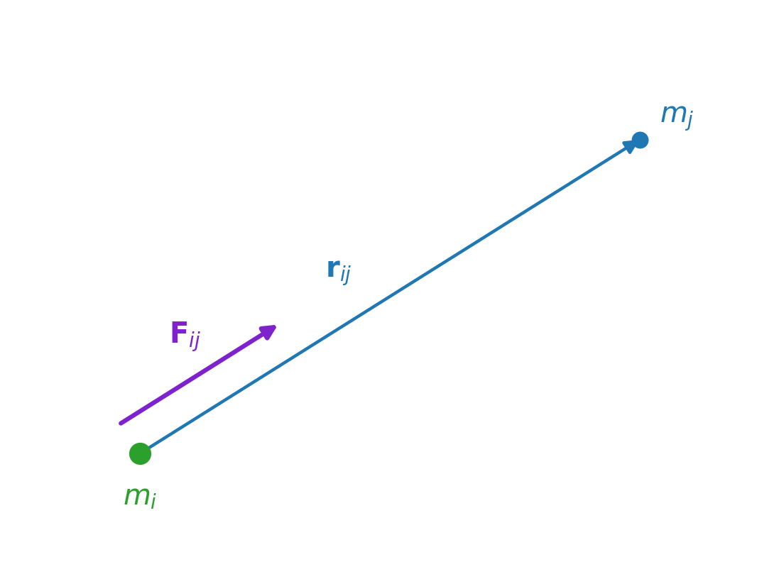
Lets consider two point masses \(m_i\) and \(m_j\) separated by a distance \(r_{ij}\), where \(\mathbf{r}_{ij}\) is the vector pointing from \(m_i\) to \(m_j\). Clearly, \(\mathbf{r}_{ij} = \mathbf{r}_j - \mathbf{r}_i\) and \(r_{ij} = |\mathbf{r}_{ij}|\). The unit vector pointing from \(m_i\) to \(m_j\) is given by \(\hat{\mathbf{r}}_{ij} = \mathbf{r}_{ij}/r_{ij}\).
The gravitational force on \(m_i\) due to \(m_j\) (in inertial frame) is given by
\[
\mathbf{F}_{ij} = G \frac{m_i m_j}{r_{ij}^{2}}\, \hat{\mathbf{r}}_{ij}, \qquad \hat{\mathbf{r}}_{ij} = \frac{\mathbf{r}_{ij}}{r_{ij}}
\]
\(G = 6.674 \times 10^{-11} \text{ m}^3 \text{ kg}^{-1} \text{ s}^{-2}\) is the gravitational constant
The sign is positive because gravity is attractive and \(\hat{\mathbf{r}}_{ij}\) already points from \(m_i\) towards \(m_j\). Many texts carry a minus sign here; they measure the unit vector in the opposite sense, from the attracting body towards the one being pulled.
Solar System Model
So we have arrived at a point mass model of the solar system, where each body is represented as a point mass. This leads to the n-body problem, where we have \(n\) point masses interacting with each other through Newton’s law of gravitation.
What is a good inertial reference frame to use for the solar system?
Answer
None exactly — every frame we can actually build is accelerating. In practice one takes the origin at the solar-system barycentre and the axes fixed to distant quasars (the ICRF).
The barycentre beats the Sun’s centre because the Sun itself orbits it, mostly under Jupiter, by up to about one solar radius. That frame is still falling towards the galactic centre at \(\sim 2\times10^{-10}\ \mathrm{m\,s^{-2}}\) — but the galactic field is very nearly uniform across the solar system, so it cancels out of the relative motion and never shows up in the dynamics we care about. “Inertial” always means inertial enough for the accuracy you need.
For the time being, we will use the Sun as the origin of our inertial reference frame. We will also assume that the Sun is stationary, and that the planets are moving in the gravitational field of the Sun.
Solar System Model (contd.)
If I apply Newton’s second law to the \(i\)-th body, I get
\[
m_i \ddot{\mathbf{R}}_i = \sum_{j=1, j\neq i}^{n} \mathbf{F}_{ij} = G \sum_{j=1, j\neq i}^{n} \frac{m_i m_j}{r_{ij}^{2}}\, \hat{\mathbf{r}}_{ij}, \qquad i = 1, 2, \ldots, n
\]
Since \(\mathbf{r}_{ij} = -\mathbf{r}_{ji}\),
\[
\sum_{i=1}^n m_i \ddot{\mathbf{R}}_i = G \sum_{i=1}^n \sum_{j=1, j\neq i}^{n} \frac{m_i m_j}{r_{ij}^{2}}\, \hat{\mathbf{r}}_{ij} = 0
\]
Integrating this equation once, we get
\[
\sum_{i=1}^n m_i \dot{\mathbf{R}}_i = \mathbf{C}_1
\]
Integarting again we get,
\[
\sum_{i=1}^n m_i \mathbf{R}_i = \mathbf{C}_1 t + \mathbf{C}_2
\]
Since by definition, the center of mass of the system is given by
\[
\mathbf{R}_{\text{cm}} = \frac{1}{M} \sum_{i=1}^n m_i \mathbf{R}_i, \qquad M = \sum_{i=1}^n m_i
\]
we conclude that the center of mass of the system moves with a constant velocity, and hence we can choose an inertial reference frame such that the center of mass is stationary.
Now taking vector cross product of the equation of motion with \(\mathbf{R}_i\), we get
\[
\sum_{i=1}^n m_i \mathbf{R}_i \times \ddot{\mathbf{R}}_i = G \sum_{i=1}^n \sum_{j=1, j\neq i}^{n} \frac{m_i m_j}{r_{ij}^{2}}\, \mathbf{R}_i \times \hat{\mathbf{r}}_{ij}
\]
Since,
\[
\mathbf{R}_{i} \times \hat{\mathbf{r}}_{ij} = \mathbf{R}_i \times \frac{\mathbf{R}_j - \mathbf{R}_i}{|\mathbf{R}_j - \mathbf{R}_i|} = \frac{\mathbf{R}_i \times \mathbf{R}_j - \mathbf{R}_i \times \mathbf{R}_i}{|\mathbf{R}_j - \mathbf{R}_i|} = \frac{\mathbf{R}_i \times \mathbf{R}_j}{|\mathbf{R}_j - \mathbf{R}_i|}
\]
and similarly,
\[
\mathbf{R}_{j} \times \hat{\mathbf{r}}_{ji} = \mathbf{R}_j \times \frac{\mathbf{R}_i - \mathbf{R}_j}{|\mathbf{R}_i - \mathbf{R}_j|} = \frac{\mathbf{R}_j \times \mathbf{R}_i - \mathbf{R}_j \times \mathbf{R}_j}{|\mathbf{R}_i - \mathbf{R}_j|} = -\frac{\mathbf{R}_i \times \mathbf{R}_j}{|\mathbf{R}_i - \mathbf{R}_j|}
\]
Therefore, we have
\[
\sum_{i=1}^n m_i \mathbf{R}_i \times \ddot{\mathbf{R}}_i = 0
\]
Integrating this equation once, we get
\[
\mathbf{H} = \sum_{i=1}^n m_i \mathbf{R}_i \times \dot{\mathbf{R}}_i = \mathbf{C}_3
\]
Therefore angular momentum of the system is conserved. That means the total angular momentum is constant in both magnitude and direction.
The plane passing through \(\mathbf{R}_{\text{cm}}\) and perpendicular to \(\mathbf{H}\) is called the invariable plane or Laplace plane. For the solar system, the invariable plane is inclined at an angle of \(1.57^\circ\) to the ecliptic plane. and \(23.44^\circ\) to the equatorial plane of the Sun.
Ecliptic plane: The plane of the Earth’s orbit around the Sun.
Equatorial plane: The plane perpendicular to the axis of rotation of the Sun. This hypothetical plane extends to infinity and is perpendicular to the Sun’s axis of rotation.
Solar System Invariable Plane
Solar-system invariable plane: the ecliptic plane, the total angular-momentum vector \(\mathbf{H}\), and the slightly tilted invariable plane defined by \(\mathbf{H}\). Planetary orbit rings are shown with exaggerated vertical scale for visibility.
This figure is highly exaggerated in the vertical direction to show the tilt of the invariable plane with respect to the ecliptic plane. The actual tilt is only \(1.57^\circ\).
Solar System Model (contd.)
We now show that the gravitational force is the gradient of a scalar.
Throughout, the gradient is taken with respect to the position of the body that feels the force, holding the source fixed:
\[
\nabla_i \equiv \frac{\partial}{\partial \mathbf{R}_i}
\]
Let \(X_{ik}\) denote the \(k^{th}\) Cartesian component of \(\mathbf{R}_i\). That is \(\mathbf{R}_i = X_{i1} \hat{i} + X_{i2} \hat{j} + X_{i3} \hat{k}\). Then
\[
r_{ij}^{2} = \mathbf{r}_{ij} \cdot \mathbf{r}_{ij} = \sum_{k=1}^{3} \left( X_{jk} - X_{ik} \right)^{2}
\]
Differentiating both sides with respect to \(X_{ik}\),
\[
2 r_{ij} \frac{\partial r_{ij}}{\partial X_{ik}} = 2 \left( X_{jk} - X_{ik} \right) (-1)
\qquad \Longrightarrow \qquad
\frac{\partial r_{ij}}{\partial X_{ik}} = -\frac{X_{jk} - X_{ik}}{r_{ij}}
\]
Collecting the three components,
\[
\nabla_i\, r_{ij} = -\frac{\mathbf{r}_{ij}}{r_{ij}} = -\hat{\mathbf{r}}_{ij}
\]
Applying the chain rule once more,
\[
\frac{\partial}{\partial X_{ik}} \left( \frac{1}{r_{ij}} \right)
= -\frac{1}{r_{ij}^{2}} \frac{\partial r_{ij}}{\partial X_{ik}}
= \frac{X_{jk} - X_{ik}}{r_{ij}^{3}}
\qquad \Longrightarrow \qquad
\nabla_i \left( \frac{1}{r_{ij}} \right) = \frac{\mathbf{r}_{ij}}{r_{ij}^{3}} = \frac{\hat{\mathbf{r}}_{ij}}{r_{ij}^{2}}
\]
Therefore,
\[
\mathbf{F}_{ij}
= \frac{G m_i m_j}{r_{ij}^{2}} \hat{\mathbf{r}}_{ij}
= \frac{G m_i m_j}{r_{ij}^{3}} \mathbf{r}_{ij}
= \nabla_i \left( \frac{G m_i m_j}{r_{ij}} \right)
= -\nabla_i \Phi_{ij},
\qquad \Phi_{ij} = -\frac{G m_i m_j}{r_{ij}}
\]
\(\Phi_{ij}\) is the mutual potential energy of the pair; note that it carries both masses. The gravitational potential of \(m_j\) — a field, defined per unit mass — is \(\phi_j = -G m_j / r_{ij}\), so that \(\Phi_{ij} = m_i \phi_j\).
Now the total force on the \(i^{th}\) body is
\[
\mathbf{F}_i = \sum_{j=1, j\neq i}^{n} \mathbf{F}_{ij} = - \sum_{j=1, j\neq i}^{n} \nabla_i \Phi_{ij} = - \nabla_i \sum_{j=1, j\neq i}^{n} \Phi_{ij} = - \nabla_i \Phi_i
\]
The equation of motion of the \(i^{th}\) body becomes
\[
m_i \ddot{\mathbf{R}}_i = \mathbf{F}_{i} = -\nabla_i \Phi_i,
\qquad
\Phi_i = \sum_{j=1, j\neq i}^{n} \Phi_{ij} = -G \sum_{j=1, j\neq i}^{n} \frac{m_i m_j}{r_{ij}}
\]
The force is the gradient of a scalar, so gravitation is a conservative force.
Take the dot product with \(\dot{\mathbf{R}}_i\) and sum over all the bodies:
\[
\sum_{i=1}^n m_i \dot{\mathbf{R}}_i \cdot \ddot{\mathbf{R}}_i = -\sum_{i=1}^n \dot{\mathbf{R}}_i \cdot \nabla_i \Phi_i
\]
The left-hand side is an exact time derivative,
\[
\sum_{i=1}^n m_i \dot{\mathbf{R}}_i \cdot \ddot{\mathbf{R}}_i
= \frac{d}{dt} \left( \frac{1}{2} \sum_{i=1}^n m_i \dot{\mathbf{R}}_i \cdot \dot{\mathbf{R}}_i \right) = \frac{dT}{dt}
\] For the right-hand side, define the potential energy of the system as a sum over pairs, not over bodies:
\[
V = -G \sum_{\text{pairs } (i,j)} \frac{m_i m_j}{r_{ij}}
= -\frac{G}{2} \sum_{i=1}^{n} \sum_{j=1, j\neq i}^{n} \frac{m_i m_j}{r_{ij}}
= \frac{1}{2} \sum_{i=1}^{n} \Phi_i
\]
\(V\) depends on time only through the positions, so by the chain rule
\[
\frac{dV}{dt} = \sum_{i=1}^{n} \nabla_i V \cdot \dot{\mathbf{R}}_i
\]
The terms of \(V\) that contain \(\mathbf{R}_i\) are those with \(k=i\) or \(l=i\) in the double sum, and they are equal in pairs, so the \(\tfrac{1}{2}\) is cancelled exactly:
\[
\nabla_i V = -G \sum_{j=1, j\neq i}^{n} m_i m_j \nabla_i \left( \frac{1}{r_{ij}} \right) = \nabla_i \Phi_i
\]
Therefore
\[
\frac{dT}{dt} = -\sum_{i=1}^{n} \dot{\mathbf{R}}_i \cdot \nabla_i V = -\frac{dV}{dt}
\]
we have
\[
\frac{d}{dt} (T + V) = 0
\]
Potential energy: It is total work done in assembling the \(n\) particales from infinite dispersion to the given configuration.
Integrating this equation, we get
\[
T + V = C_4
\]
Note on Conservative Force
Now, \[
\Phi_{ij} = -\frac{G m_i m_j}{r_{ij}}, \qquad \mathbf{F}_{ij} = -\nabla_i \Phi_{ij} = G m_i m_j\,\frac{\mathbf{r}_{ij}}{r_{ij}^{3}}.
\]
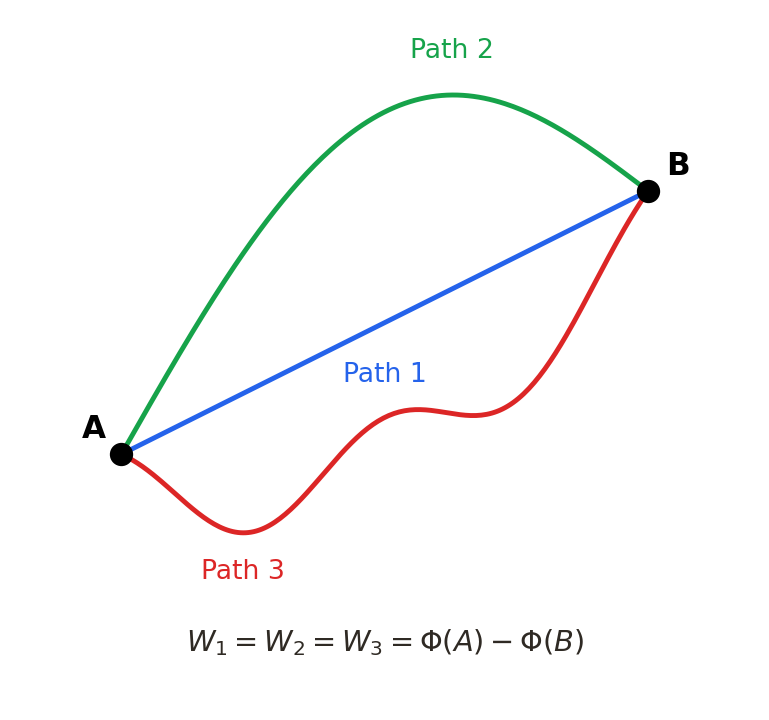
If I have to move a point mass from point A to point B, the work done by the gravitational field is
\[ W = \int_A^B \mathbf F_{ij}\cdot d\mathbf r = \Phi(A) - \Phi(B). \]
This means the work done is independent of the path taken between A and B.
Clearly,
\[\nabla_i \times \mathbf F_{ij} = -\nabla_i \times (\nabla_i \Phi_{ij}) = 0.\]
Hence, the gravitational field is irrotational.
We note here that force is a vector quantity, while the potential is a scalar quantity. Therefore, it is easier to work with the potential than the force when dealing with multiple masses.
Does this mean that if I move a satellite from one orbit to another orbit, any path that I take will have the same work done?
Answer
Yes for the work, no for the fuel — and the gap between those two is where mission design lives.
Gravity is conservative, so \(W_{\text{grav}} = -\Delta U\) depends only on the endpoints; and since the initial and final orbits fix \(\varepsilon\) at each end, the energy the engine must supply is fixed too.
What is not fixed is the \(\Delta v\) — the propellant — needed to deliver it. A tangential impulse buys \(\Delta\varepsilon = v\,\Delta v + \tfrac{1}{2}\Delta v^{2}\), so the same energy costs less \(\Delta v\) where \(v\) is already large. Burn placement, plane changes and finite-burn losses all move the bill even though the work does not.
Irrotationality of \(\mathbf g\) — directly
We can also show \(\nabla\times\mathbf g = \mathbf 0\) without the potential. For a point mass \(M\) at the origin,
\[
\mathbf g = -GM\,\frac{\mathbf r}{r^{3}}, \qquad r = \sqrt{x^2+y^2+z^2}, \qquad \frac{\partial r}{\partial x} = \frac{x}{r}.
\]
Take the \(z\)-component of the curl (the \(x,y\) components follow by symmetry):
\[
(\nabla\times\mathbf g)_z = \frac{\partial g_y}{\partial x} - \frac{\partial g_x}{\partial y}.
\]
Each partial gives the same mixed term, so they cancel:
\[
\frac{\partial g_y}{\partial x}
= -GM\,\frac{\partial}{\partial x}\!\left(\frac{y}{r^{3}}\right)
= \frac{3GM\,xy}{r^{5}}
= -GM\,\frac{\partial}{\partial y}\!\left(\frac{x}{r^{3}}\right)
= \frac{\partial g_x}{\partial y}.
\]
Hence \((\nabla\times\mathbf g)_z = 0\), and likewise for the other components:
\[
\boxed{\;\nabla\times\mathbf g = \mathbf 0\;}
\]
More generally, any central field \(\mathbf g = g(r)\,\hat{\mathbf r}\) is irrotational, because \(\nabla g(r) = g'(r)\,\hat{\mathbf r}\) is parallel to \(\hat{\mathbf r}\).
Solution of N-body Problem
The governing dynamical equations are:
\[
m_i \ddot{\mathbf{R}}_i = G \sum_{j=1, j\neq i}^{n} \frac{m_i m_j}{r_{ij}^{2}}\, \hat{\mathbf{r}}_{ij}, \qquad i = 1, 2, \ldots, n
\]
Coupled with the kinematic equations
\[
\dot{\mathbf{R}}_i = \mathbf{V}_i, \qquad i = 1, 2, \ldots, n
\]
they form the complete state of the system. The initial conditions are given by
\[
\mathbf{R}_i(0) = \mathbf{R}_{i0}, \qquad \mathbf{V}_i(0) = \mathbf{V}_{i0}, \qquad i = 1, 2, \ldots, n
\]
We note here that for a N-body system, there are 6N first order ODEs, and hence we need 6N initial conditions to solve the system.
For analytical solutions to exist, we need to have \(6N\) independent integrals of motion. We have already seen that we have 10 integrals of motion, which are the total energy (\(C_4\)), the initial position of the center of mass (\(C_2\)), the initial velocity of the center of mass (\(C_1\)), and the total angular momentum conservation (\(C_3\)). Therefore, we have 10 integrals of motion, which is less than \(6N\) for \(N \ge 2\).
In case of \(N = 2\), we have 12 initial conditions, and hence we need 12 independent integrals of motion. We have 10 classical integrals of motion, coupled with the elimination of the time and the node, reduce the system from order \(6N\) to order \(6N - 12\). Hence, analytical solutions exist for \(N = 2\).
However, analytical solutions do not exist for \(N > 3\).
Numerical Solution of 3-body Problem
- Any standard ODE integrator can be used to solve the 3-body problem numerically.
![]()
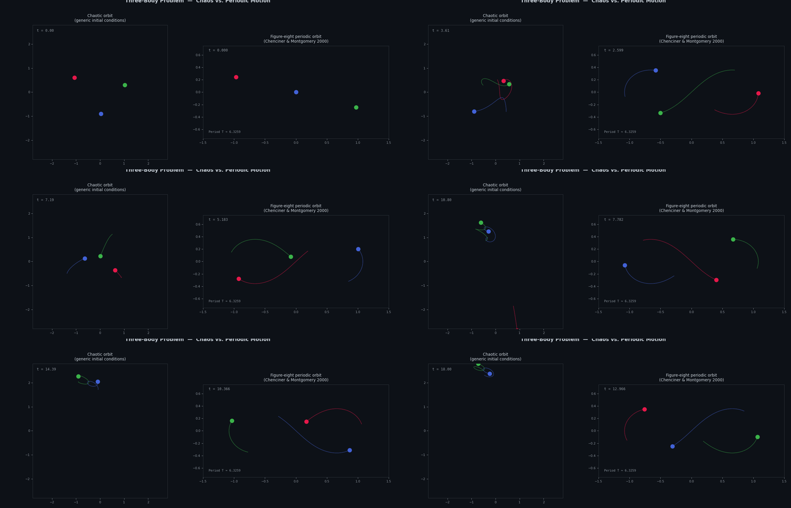
Figure 3: Animation of the three-body problem: chaotic orbit (left) vs. figure-eight periodic orbit (right). Download the script.
The left panel shows a chaotic orbit. Precise definition is beyond the scope of this course, but it is a trajectory that is highly sensitive to initial conditions. A small change in the initial conditions can lead to a completely different trajectory. The solar system is chaotic, but the time scale for this chaos to manifest is very long, around 5 million years.
Secondly, the right panel shows a periodic orbit, which is a special solution of the three-body problem. The figure-eight orbit is one of the very few exact periodic solutions known for the three-body problem. Both cases use equal masses and G = 1 (non-dimensional units).