The Two-Body Problem
Integrals, conics, velocity and time on every Kepler orbit
1 Where we are going
The \(N\)-body note ended with a problem and a way out. The problem: for three or more bodies the equations of motion have no general closed-form solution. The way out: the masses in the solar system are extremely uneven, so most of the time one body moves under the pull of one other body, and everything else is a small disturbance. This note solves that problem, the two-body problem, completely.
It is worth knowing in advance how much comes out of it. From a single vector equation we will obtain Kepler’s three laws, the shape of every possible orbit, the speed and direction of motion at every point, the condition for escape, the bending of a flyby, and the position of the body at any time. Almost every calculation in the rest of the course starts from a formula derived here.
As in the \(N\)-body note, two kinds of boxes run through the text. A blue Try it box asks you to do something small: compute a number, check a step, play with a figure. A green Check yourself box asks a short question about what you have just read. Each has a hidden answer; open it only after you have one of your own.
1.1 The plan, and the one place where the conics part company
The note is in two halves, and it pays to see the split before starting.
Section 2: what every orbit shares. The equation of motion, its three integrals (angular momentum \(\mathbf h\), the eccentricity vector \(\mathbf e\) and the energy \(\varepsilon\)), the shape of the orbit, the energy equation, the velocity, the flight path angle and the hodograph. None of these derivations needs to know whether the orbit is a circle, an ellipse, a parabola or a hyperbola. They hold for all four.
Section 3, Section 4 and Section 5: where the conics part company. Only one question forces us to treat the conics separately: where is the body at time \(t\)? Answering it needs an integral that is evaluated differently for each conic, and a handful of quantities (the farthest point, the period, the speed at infinity) that exist for some conics and not for others.
Section 6 puts the conics side by side, and an appendix (Section 7) proves two kinematic formulas used along the way.
When you finish, you should be able to answer the following without hand-waving.
- Why is the relative motion of two bodies confined to a plane, and why is the orbit a conic section?
- Why does the energy of an orbit depend only on its size and not on its shape?
- What is the escape speed, and why is it a speed and not a velocity?
- What are the speed and the direction of flight at any point of any orbit?
- Given the time, how do you find the position on an ellipse, a parabola and a hyperbola, and why is this so much harder than finding the shape?
- How much does a flyby turn a spacecraft, and what decides it?
2 What every orbit shares
2.1 From two bodies to one
2.1.1 The relative equation of motion
Take \(n=2\) in the \(N\)-body equations. With \(\mathbf r_{12}=\mathbf R_2-\mathbf R_1\) (the vector from body 1 to body 2) and \(r_{12}=|\mathbf r_{12}|\), the two equations of motion, divided by the masses, are
\[ \ddot{\mathbf R}_1=\frac{Gm_2}{r_{12}^{3}}\,\mathbf r_{12},\qquad \ddot{\mathbf R}_2=\frac{Gm_1}{r_{12}^{3}}\,\mathbf r_{21}=-\frac{Gm_1}{r_{12}^{3}}\,\mathbf r_{12}. \]
The \(N\)-body note told us that what matters is the relative motion, so subtract the first from the second:
\[ \ddot{\mathbf r}_{12}=\ddot{\mathbf R}_2-\ddot{\mathbf R}_1 =-\frac{Gm_1}{r_{12}^{3}}\,\mathbf r_{12}-\frac{Gm_2}{r_{12}^{3}}\,\mathbf r_{12} =-\frac{G(m_1+m_2)}{r_{12}^{3}}\,\mathbf r_{12}. \]
Something good has happened: the right-hand side contains only \(\mathbf r_{12}\). The relative position obeys an equation of its own, which no longer involves \(\mathbf R_1\) or \(\mathbf R_2\) separately. Dropping the subscripts, writing \(\mathbf r\) for \(\mathbf r_{12}\) and \(r=|\mathbf r|\),
\[ \ddot{\mathbf r}+\frac{\mu}{r^{3}}\,\mathbf r=\mathbf 0,\qquad \mu=G(m_1+m_2). \tag{1}\]
This is the two-body equation of motion, and the rest of the note is about its solutions. The constant \(\mu\) is the gravitational parameter of the pair. Only \(\mu\) appears, not the two masses separately: to predict the relative motion we never need to know \(G\), \(m_1\) or \(m_2\) on their own.
History: why astronomers quote \(\mu\). Orbits measure \(\mu\) directly, through Kepler’s third law, while \(G\) must be measured in a laboratory, with small masses and tiny forces. So \(\mu\) is known far better than \(G\): \(GM_\oplus=398\,600.4418\pm0.0008\) km\(^3\)/s\(^2\) (two parts in \(10^{9}\)), whereas \(G\) itself is known only to about two parts in \(10^{5}\). Since the Sun outweighs every planet by at least a factor of a thousand, astronomers could compute planetary orbits accurately long before anyone knew the planets’ masses, or the Sun’s.
Weigh the Sun. For the Earth’s orbit, \(a=1\) AU \(=1.496\times10^{8}\) km and the period is one sidereal year, \(365.256\) days. Kepler’s third law in Newton’s form (proved in Section 3.3) is \(T=2\pi\sqrt{a^3/\mu}\). Solve for \(\mu\).
What you should find
\(\mu=4\pi^2a^3/T^2=1.327\times10^{11}\) km\(^3\)/s\(^2\). This is \(G(M_\odot+M_\oplus)\), which to six figures is \(GM_\odot\). To get the mass in kilograms you would still need \(G\), and that is the weak link.2.1.2 Recovering the two bodies
Equation 1 gives the relative motion. Where are the bodies themselves? The answer combines it with the centre of mass, which moves uniformly (the \(N\)-body note). Write \(M=m_1+m_2\) and
\[ \mathbf R_{\rm cm}=\frac{m_1}{M}\mathbf R_1+\frac{m_2}{M}\mathbf R_2,\qquad \mathbf r=-\mathbf R_1+\mathbf R_2 . \]
This is a linear change of variables, \((\mathbf R_1,\mathbf R_2)\mapsto(\mathbf R_{\rm cm},\mathbf r)\), acting in the same way on each Cartesian component:
\[ \begin{pmatrix}\mathbf R_{\rm cm}\\ \mathbf r\end{pmatrix} =\underbrace{\begin{pmatrix}m_1/M & m_2/M\\ -1 & 1\end{pmatrix}}_{A} \begin{pmatrix}\mathbf R_1\\ \mathbf R_2\end{pmatrix}, \qquad \det A=\frac{m_1}{M}+\frac{m_2}{M}=1 . \]
Since \(\det A\ne0\) the change can be undone. Inverting the \(2\times2\) matrix,
\[ A^{-1}=\begin{pmatrix}1 & -m_2/M\\ 1 & m_1/M\end{pmatrix}, \]
that is,
\[ \boxed{\;\begin{aligned}\mathbf R_1&=\mathbf R_{\rm cm}-\frac{m_2}{M}\,\mathbf r,\\[2pt] \mathbf R_2&=\mathbf R_{\rm cm}+\frac{m_1}{M}\,\mathbf r .\end{aligned}\;} \tag{2}\]
Differentiating gives the velocities in the same way. So the recipe is: solve Equation 1 for \(\mathbf r(t)\), move the centre of mass uniformly, and combine them with Equation 2.
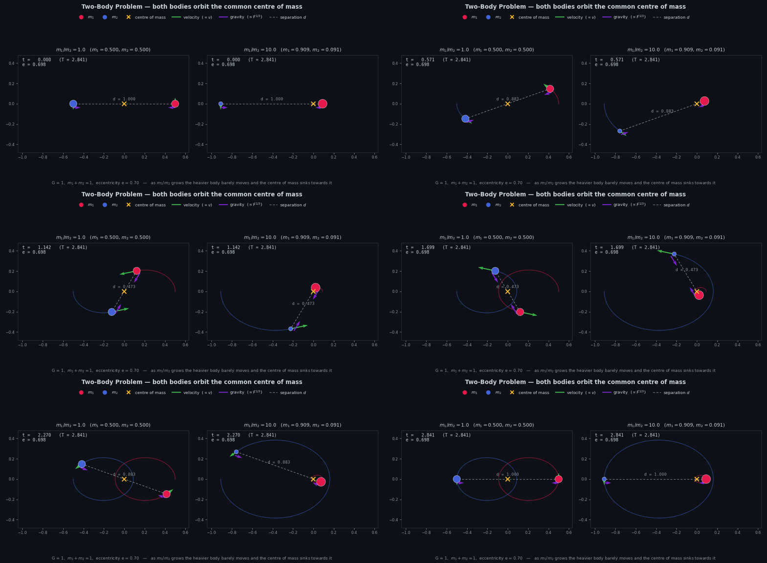
In the barycentric frame, \(\mathbf R_{\rm cm}=\mathbf 0\), and Equation 2 says that both bodies are fixed multiples of the same vector \(\mathbf r(t)\): they stay on opposite sides of the barycentre, and each traces a copy of the relative orbit scaled by a constant. Figure 1 shows this.
In Equation 2, body 1 is scaled by \(m_2/M\) and body 2 by \(m_1/M\): the weights are crossed. Which body traces the smaller orbit about the barycentre? The two forces are equal and opposite; are the two accelerations?
Answer
The heavier body traces the smaller orbit: if \(m_1>m_2\) then \(m_2/M<m_1/M\). The forces are equal in size, but the accelerations are not, since \(|\ddot{\mathbf R}_1|/|\ddot{\mathbf R}_2|=m_2/m_1\). The heavier body responds less, and so moves less.Pluto and its moon Charon are \(19\,596\) km apart, and \(m_{\rm Charon}/m_{\rm Pluto}=0.122\). How far from the centre of Pluto is their barycentre? Pluto’s radius is \(1188\) km.
What you should find
From Equation 2 the distance is \(r\,m_C/(m_P+m_C)=19\,596\times0.122/1.122\approx2130\) km, which is outside Pluto. Pluto and Charon both orbit a point in empty space between them. Compare the Earth–Moon barycentre, \(4671\) km from the Earth’s centre, inside the Earth.As \(m_1/m_2\) grows, the orbit of the heavier body shrinks and the barycentre moves towards its centre. For the Sun and Jupiter, \(m_1/m_2\approx1047\), the Sun’s orbit about the barycentre is \(1/1047\) the size of Jupiter’s (just over a solar radius). This is the quantitative content of the restricted two-body problem: when one mass is much larger, treat it as fixed, and let \(\mathbf r\) be the position of the small body measured from the large one. Equation 1 does not change; only the interpretation of \(\mathbf r\) does, and for planets and satellites \(\mu\) is, to excellent accuracy, \(G\) times the mass of the central body.
2.2 Angular momentum: the motion is planar
Equation 1 is a nonlinear vector ODE of second order. Rather than attack it directly, we repeat the strategy of the \(N\)-body note: look for integrals, combinations of \(\mathbf r\) and \(\dot{\mathbf r}\) that do not change. The acceleration in Equation 1 is parallel to \(\mathbf r\), and the cross product of parallel vectors vanishes, so the first thing to try is a cross product with \(\mathbf r\):
\[ \mathbf r\times\ddot{\mathbf r}=-\frac{\mu}{r^3}\,\mathbf r\times\mathbf r=\mathbf 0 . \]
The left-hand side is an exact derivative, because
\[ \frac{d}{dt}\left(\mathbf r\times\dot{\mathbf r}\right)=\dot{\mathbf r}\times\dot{\mathbf r}+\mathbf r\times\ddot{\mathbf r}=\mathbf r\times\ddot{\mathbf r}. \]
Therefore the specific angular momentum (angular momentum per unit mass)
\[ \mathbf h=\mathbf r\times\dot{\mathbf r} \tag{3}\]
is a constant vector. Three scalar constants.
What it implies. At every instant \(\mathbf r\cdot\mathbf h=\mathbf r\cdot(\mathbf r\times\dot{\mathbf r})=0\), since a triple product with a repeated vector vanishes. So \(\mathbf r(t)\) is always perpendicular to \(\mathbf h\). Since \(\mathbf h\) does not change, \(\mathbf r(t)\) lies for all time in one fixed plane through the origin, the plane perpendicular to \(\mathbf h\). The relative motion is planar.
This is a strong geometric statement. A curve in three dimensions has collapsed into a curve in a plane, and from now on we can do orbital geometry in two dimensions.
Is \(h=0\) possible? If yes, what kind of motion results?
Answer
Yes. \(\mathbf h=\mathbf r\times\dot{\mathbf r}=\mathbf 0\) exactly when \(\mathbf r\) and \(\dot{\mathbf r}\) are parallel, and then the motion is rectilinear: a straight line through the centre of attraction. Dropping a body from rest is the standard example. The argument above then fails (there is no normal to define a plane), and correctly so: every plane that contains the line will do. We will meet this case again; it is the one orbit that the formulas of this note describe badly.Kepler’s second law. In the orbital plane, use polar coordinates \((r,\theta)\) centred on the attracting body. In a short time \(dt\) the radius vector sweeps a thin triangle of area \(dA=\tfrac12r^2\,d\theta\), and \(|\mathbf h|=r^2\dot\theta\) (we prove this in Section 2.11; the transverse component of the velocity is \(r\dot\theta\)). So
\[ \frac{dA}{dt}=\frac12r^2\dot\theta=\frac h2=\text{constant}. \]
Equal areas in equal times: Kepler’s second law is the conservation of angular momentum.
Kepler’s second law holds for any central force, not only for the inverse square. Why?
Answer
The only property of the force used above was that \(\ddot{\mathbf r}\) is parallel to \(\mathbf r\), so that \(\mathbf r\times\ddot{\mathbf r}=\mathbf 0\). Any force directed along \(\mathbf r\), whatever its dependence on \(r\), conserves \(\mathbf h\), and with it the areal velocity. The second law tells you the force is central; it does not tell you it is an inverse square. The first and third laws do.2.3 The eccentricity vector: the orbit does not turn
Angular momentum fixes the plane of the orbit. It does not tell us whether the orbit keeps a fixed orientation inside that plane, or slowly turns. Is there a second vector integral, one that lies in the plane and points in a fixed direction?
Here is the idea. We want to integrate Equation 1, and the obstacle is the right-hand side \(-\mu\mathbf r/r^3\), which is not obviously the derivative of anything. Since \(\mathbf h\) is constant, \(\ddot{\mathbf r}\times\mathbf h\) is an exact derivative, of \(\dot{\mathbf r}\times\mathbf h\). So take the cross product of Equation 1 with \(\mathbf h\) and hope that the right-hand side becomes a derivative too.
\[ \ddot{\mathbf r}\times\mathbf h=-\frac{\mu}{r^3}\,\mathbf r\times\mathbf h =-\frac{\mu}{r^3}\,\mathbf r\times\left(\mathbf r\times\dot{\mathbf r}\right). \]
Expand the triple product with \(\mathbf a\times(\mathbf b\times\mathbf c)=(\mathbf a\cdot\mathbf c)\mathbf b-(\mathbf a\cdot\mathbf b)\mathbf c\):
\[ \ddot{\mathbf r}\times\mathbf h =-\frac{\mu}{r^3}\left[(\mathbf r\cdot\dot{\mathbf r})\,\mathbf r-(\mathbf r\cdot\mathbf r)\,\dot{\mathbf r}\right] =-\frac{\mu}{r^3}\left[(\mathbf r\cdot\dot{\mathbf r})\,\mathbf r-r^2\,\dot{\mathbf r}\right]. \]
We need \(\mathbf r\cdot\dot{\mathbf r}\). Write \(\mathbf r=r\hat{\mathbf r}\), where \(\hat{\mathbf r}\) is the unit vector along \(\mathbf r\). Then \(\dot{\mathbf r}=\dot r\,\hat{\mathbf r}+r\,\dot{\hat{\mathbf r}}\) and
\[ \mathbf r\cdot\dot{\mathbf r}=r\hat{\mathbf r}\cdot\left(\dot r\,\hat{\mathbf r}+r\,\dot{\hat{\mathbf r}}\right) =r\dot r\,(\hat{\mathbf r}\cdot\hat{\mathbf r})+r^2\,(\hat{\mathbf r}\cdot\dot{\hat{\mathbf r}})=r\dot r, \]
because \(\hat{\mathbf r}\cdot\hat{\mathbf r}=1\) and, differentiating that, \(\hat{\mathbf r}\cdot\dot{\hat{\mathbf r}}=0\). (Note that \(\dot r\), the rate of change of the distance, is not the same as \(|\dot{\mathbf r}|\), the speed.) Substituting,
\[ \ddot{\mathbf r}\times\mathbf h=-\frac{\mu}{r^3}\left[r\dot r\,\mathbf r-r^2\dot{\mathbf r}\right] =\mu\left(\frac{\dot{\mathbf r}}{r}-\frac{\dot r}{r^2}\,\mathbf r\right). \]
The bracket is exactly the derivative of the unit vector \(\mathbf r/r\), by the quotient rule:
\[ \frac{d}{dt}\left(\frac{\mathbf r}{r}\right)=\frac{\dot{\mathbf r}}{r}-\frac{\dot r}{r^2}\,\mathbf r . \]
So the hope came true: \(\ddot{\mathbf r}\times\mathbf h=\mu\,\dfrac{d}{dt}\left(\dfrac{\mathbf r}{r}\right)\). Both sides are exact derivatives, and integrating once,
\[ \dot{\mathbf r}\times\mathbf h=\mu\left(\frac{\mathbf r}{r}+\mathbf e\right), \qquad\text{i.e.}\qquad \mathbf e=\frac{\dot{\mathbf r}\times\mathbf h}{\mu}-\frac{\mathbf r}{r}, \tag{4}\]
where \(\mathbf e\) is a constant vector of integration. It is dimensionless (each term on the right is), and it is called the eccentricity vector, for reasons that will be clear in Section 2.4.
Since \(\mathbf e\) arose as a constant of integration, its constancy is built in. As a check, differentiate Equation 4 using \(\dot{\mathbf h}=\mathbf 0\):
\[ \dot{\mathbf e}=\frac{\ddot{\mathbf r}\times\mathbf h}{\mu}-\frac{d}{dt}\left(\frac{\mathbf r}{r}\right)=\mathbf 0, \]
by the identity just proved. A constant vector has a constant length \(e=|\mathbf e|\) and a constant direction. So \(\mathbf e\) singles out one fixed line in the orbital plane, for all time. We will see in a moment that it points to the point of closest approach, and that \(e\) is the eccentricity of the orbit.
Show that \(\mathbf e\) lies in the orbital plane, i.e. \(\mathbf h\cdot\mathbf e=0\). Then compute \(\mathbf e\cdot\dot{\mathbf r}\). Is \(\mathbf e\) perpendicular to the velocity?
What you should find
\(\mathbf h\cdot(\dot{\mathbf r}\times\mathbf h)=0\) (repeated vector in a triple product) and \(\mathbf h\cdot\mathbf r=0\), so \(\mathbf h\cdot\mathbf e=0\).
For the velocity, \(\dot{\mathbf r}\cdot(\dot{\mathbf r}\times\mathbf h)=0\) too, but \(\dot{\mathbf r}\cdot\mathbf r/r=r\dot r/r=\dot r\). Hence \(\mathbf e\cdot\dot{\mathbf r}=-\dot r\). This vanishes only where the distance is momentarily stationary (the closest and farthest points). So \(\mathbf e\) is perpendicular to \(\mathbf h\) always, but perpendicular to \(\dot{\mathbf r}\) only at those two points. A common mistake is to claim the second.Why it matters. \(\mathbf h\) fixes the orbital plane; \(\mathbf e\) fixes the orientation of the orbit within the plane. Its constancy is the statement that the orbit does not precess: the closed curve that we are about to find returns exactly on itself, revolution after revolution. That is a special property of the inverse-square law. Any departure from \(1/r^2\) (the Earth’s oblateness, the pull of a third body, the corrections of general relativity) makes \(\dot{\mathbf e}\ne\mathbf 0\), and the line through the closest and farthest points, the line of apsides, slowly rotates. This rotation is called apsidal precession. The best-known case is Mercury: after all the Newtonian perturbations of the other planets are accounted for, its line of apsides still turns by an extra \(43''\) per century, which general relativity explains exactly.
History: many names for one vector. The vector \(\mu\mathbf e\) is often called the Laplace–Runge–Lenz vector. Laplace used it in his Traité de mécanique céleste (1799), but it appears already in a 1710 exchange between Jakob Hermann and Johann Bernoulli. Carl Runge put it in a textbook on vector analysis, Wilhelm Lenz used it in 1924 for the old quantum theory of the hydrogen atom, and Wolfgang Pauli then used it to derive the hydrogen spectrum, which made it famous among physicists. (H. Goldstein, Am. J. Phys. 1975 and 1976, traces the history.)
2.4 The orbit equation
We now have two constant vectors, \(\mathbf h\) (normal to the plane) and \(\mathbf e\) (in the plane). That is enough to find the shape of the orbit without solving any differential equation. The trick is to take a dot product that turns Equation 4 into a scalar relation involving only \(r\) and one angle.
Take the dot product of \(\mathbf r\) with the first form of Equation 4, \(\dot{\mathbf r}\times\mathbf h=\mu(\hat{\mathbf r}+\mathbf e)\). On the left, cycle the triple product:
\[ \mathbf r\cdot\left(\dot{\mathbf r}\times\mathbf h\right)=\mathbf h\cdot\left(\mathbf r\times\dot{\mathbf r}\right)=\mathbf h\cdot\mathbf h=h^2 . \]
On the right, define the true anomaly \(f\) as the angle from \(\mathbf e\) to \(\mathbf r\), measured in the direction of motion. Then \(\mathbf r\cdot\mathbf e=re\cos f\) and
\[ \mathbf r\cdot\mu\left(\hat{\mathbf r}+\mathbf e\right)=\mu\left(r+re\cos f\right). \]
Equating the two and solving for \(r\),
\[ \boxed{\;r=\frac{p}{1+e\cos f},\qquad p=\frac{h^2}{\mu}.\;} \tag{5}\]
This is the polar equation of a conic section with the origin at a focus. The length \(p\) is called the semi-latus rectum; it is the value of \(r\) at \(f=\pm90^\circ\). The single number \(e=|\mathbf e|\) decides the type of conic:
| \(e\) | conic | |
|---|---|---|
| \(0\) | circle | closed |
| \(0<e<1\) | ellipse | closed |
| \(1\) | parabola | open |
| \(>1\) | hyperbola | open |
This is Kepler’s first law, and more: Kepler found ellipses, but the inverse-square law also allows parabolas and hyperbolas.
The direction of \(\mathbf e\). For \(e>0\), \(r\) in Equation 5 is smallest where \(1+e\cos f\) is largest, at \(f=0\). That point of closest approach is the periapsis. Since \(f\) is measured from \(\mathbf e\), we have shown:
\[ \boxed{\;\mathbf e\text{ points from the focus towards periapsis.}\;} \]
(For a closed orbit, \(r\) is largest at \(f=180^\circ\), the apoapsis. With the Earth as the central body these are called perigee and apogee; with the Sun, perihelion and aphelion.)
Two quick questions. (a) What does the orbit look like when \(\mathbf e=\mathbf 0\), and why is the direction of \(\mathbf e\) then meaningless? (b) In Equation 5, what are \(p\) and \(e\) for an orbit with \(h=0\)?
Answer
\(r=p\) for every \(f\): a circle. There is no closest point, so there is nothing for \(\mathbf e\) to point at, and the true anomaly \(f\) has no natural origin.
\(p=h^2/\mu=0\). From Equation 4 with \(\mathbf h=\mathbf 0\), \(\mathbf e=-\hat{\mathbf r}\), so \(e=1\) whatever the energy. The “conic” degenerates into a straight segment, and \((p,e)\) no longer tells you its size. This is the rectilinear orbit of the \(h=0\) question in Section 2.2.
2.4.1 Reading the orbit equation
Before any more dynamics, Equation 5 already says which values of \(f\) are allowed. Since \(r>0\) and \(p>0\), we need
\[ 1+e\cos f>0 . \]
- \(e<1\). Then \(1+e\cos f\ge1-e>0\) for every \(f\), so \(f\) runs over the whole circle and the curve closes. Both apsides exist, at \(r_p=p/(1+e)\) and \(r_a=p/(1-e)\).
- \(e=1\). The denominator vanishes only as \(f\to\pm180^\circ\), where \(r\to\infty\). The curve is open and there is no apoapsis. Periapsis is at \(r_p=p/2\).
- \(e>1\). The denominator vanishes at a finite angle \(f_\infty\), given by
\[ \cos f_\infty=-\frac1e , \tag{6}\]
and the body exists only on the arc \(|f|<f_\infty\). As \(f\to\pm f_\infty\), \(r\to\infty\): the two directions \(f=\pm f_\infty\) are the asymptotes of the hyperbola.
So the split between the conics is visible already in the geometry, and it is entirely a matter of the denominator.
As \(e\to1^{+}\), what happens to \(f_\infty\)? And as \(e\to\infty\)? Describe the trajectory in each limit.
Answer
\(f_\infty=\arccos(-1/e)\) decreases from \(180^\circ\) (at \(e=1\)) towards \(90^\circ\) (as \(e\to\infty\)). As \(e\to1^+\), the asymptotes fold back towards the line of apsides and the hyperbola approaches a parabola, which “reaches infinity” only at \(f=180^\circ\). As \(e\to\infty\), the asymptotes become perpendicular to the line of apsides and the trajectory is nearly a straight line, barely bent by the central body: a very fast flyby.2.5 Energy: the vis-viva integral
We crossed Equation 1 with \(\mathbf r\) and then with \(\mathbf h\). The remaining natural product is the dot product with the velocity, which in mechanics always produces an energy equation:
\[ \dot{\mathbf r}\cdot\ddot{\mathbf r}=-\frac{\mu}{r^3}\,\mathbf r\cdot\dot{\mathbf r}. \]
With \(v=|\dot{\mathbf r}|\), the left side is \(\frac{d}{dt}\left(\tfrac12v^2\right)\). On the right, \(\mathbf r\cdot\dot{\mathbf r}=r\dot r\) (shown in Section 2.3), so
\[ \frac{d}{dt}\left(\frac{v^2}{2}\right)=-\frac{\mu\dot r}{r^2}=\frac{d}{dt}\left(\frac{\mu}{r}\right). \]
Integrating,
\[ \boxed{\;\frac{v^2}{2}-\frac{\mu}{r}=\varepsilon\;} \tag{7}\]
where the constant \(\varepsilon\) is the specific mechanical energy: kinetic energy per unit mass (\(v^2/2\)) plus potential energy per unit mass (\(-\mu/r\)). This is the energy integral, or the vis-viva equation (Latin for “living force”, an old name for kinetic energy). It is arguably the single most useful formula in mission design: it connects speed and distance on any orbit with one constant.
2.6 Seven constants, five independent: the Casimir relations
We have squeezed Equation 1 in three ways and obtained three integrals:
\[ \mathbf h=\mathbf r\times\dot{\mathbf r},\qquad \mathbf e=\frac{\dot{\mathbf r}\times\mathbf h}{\mu}-\frac{\mathbf r}{r},\qquad \varepsilon=\frac{v^2}{2}-\frac{\mu}{r}. \]
That is \(3+3+1=7\) scalar constants. But the state \((\mathbf r,\dot{\mathbf r})\) has only \(6\) components, and the constants must not pin the state down completely (otherwise the body could not move). A system of order \(6\) has at most \(5\) independent integrals that do not involve time. So the seven constants must be tied together by at least two relations. Here they are:
\[ \boxed{\;\mathbf h\cdot\mathbf e=0\;}\qquad\qquad \boxed{\;\mu^2\left(e^2-1\right)=2\varepsilon h^2\;} \tag{8}\]
These are sometimes called the Casimir relations. Neither is a new integral; they are identities satisfied by the integrals we have, on every orbit. The first you proved in the Try-it box of Section 2.3. We prove the second.
Take the squared length of Equation 4, written as \(\mu\mathbf e=\dot{\mathbf r}\times\mathbf h-\mu\hat{\mathbf r}\):
\[ \mu^2e^2=\underbrace{\left|\dot{\mathbf r}\times\mathbf h\right|^2}_{\text{(i)}} -2\mu\,\underbrace{\hat{\mathbf r}\cdot\left(\dot{\mathbf r}\times\mathbf h\right)}_{\text{(ii)}} +\mu^2\,\underbrace{\hat{\mathbf r}\cdot\hat{\mathbf r}}_{=1}. \]
Term (i). \(\mathbf h=\mathbf r\times\dot{\mathbf r}\) is perpendicular to \(\dot{\mathbf r}\), so the cross product has magnitude \(vh\), with no sine factor: \(|\dot{\mathbf r}\times\mathbf h|^2=v^2h^2\).
Term (ii). Cycle the triple product so that \(\mathbf h\) meets \(\mathbf r\times\dot{\mathbf r}\):
\[ \hat{\mathbf r}\cdot\left(\dot{\mathbf r}\times\mathbf h\right)=\frac1r\,\mathbf h\cdot\left(\mathbf r\times\dot{\mathbf r}\right)=\frac{h^2}{r}. \]
Substituting both,
\[ \mu^2e^2=v^2h^2-\frac{2\mu h^2}{r}+\mu^2=h^2\left(v^2-\frac{2\mu}{r}\right)+\mu^2=2\varepsilon h^2+\mu^2 , \]
since the bracket is \(2\varepsilon\) by Equation 7. Rearranged, this is Equation 8, or, solved for the eccentricity,
\[ e=\sqrt{1+\frac{2\varepsilon h^2}{\mu^2}} . \tag{9}\]
Since \(h^2\ge0\), the sign of the energy alone decides the type of conic:
| energy | eccentricity | orbit |
|---|---|---|
| \(\varepsilon<0\) | \(e<1\) | ellipse (or circle) |
| \(\varepsilon=0\) | \(e=1\) | parabola |
| \(\varepsilon>0\) | \(e>1\) | hyperbola |
This is why \(\varepsilon\) is the natural mission-design variable: one number, computed from one position and one speed, tells you at a glance whether the spacecraft is captured or escaping.
Counting. Seven constants minus two relations leaves five independent constants. Five numbers fix the orbit as a curve in space: two for the orientation of the plane, one for the orientation of the line of apsides in the plane, and two for the size and shape (for example \(h\) and \(e\)). What they cannot tell us is where on the curve the body is at a given time. A sixth constant does that, for example the time \(t_p\) at which the body passes periapsis:
\[ 5\ (\text{geometry})+1\ (\text{timing, e.g. }t_p)=6, \]
which is the order of Equation 1.
The first five come from the integrals; the sixth will cost us the hardest work in the note (Section 2.14 onwards).
A spacecraft is at \(r=7000\) km from the Earth’s centre, moving at \(v=8.0\) km/s (\(\mu=398\,600\) km\(^3\)/s\(^2\)). Without knowing the direction of the velocity, can you tell whether it will escape? Can you tell its eccentricity?
Answer
\(\varepsilon=8.0^2/2-398\,600/7000=32.0-56.9=-24.9\) km\(^2\)/s\(^2<0\), so it is bound and cannot escape, whatever the direction. The eccentricity needs \(h=rv\cos\gamma\), which depends on the direction of the velocity, so \(e\) cannot be found from \(r\) and \(v\) alone.2.7 The size parameter \(a\)
The second Casimir relation, with \(h^2=\mu p\), already expresses the energy through the shape parameters alone:
\[ \mu^2\left(e^2-1\right)=2\varepsilon\,\mu p \qquad\Longrightarrow\qquad \varepsilon=\frac{\mu\left(e^2-1\right)}{2p}. \]
This is exact for every conic, but awkward: engineers quote neither \(p\) nor \(\varepsilon\), but a length. So we define one,
\[ \boxed{\;a\equiv\frac{p}{1-e^2}\;}\qquad\Longleftrightarrow\qquad\boxed{\;p=a\left(1-e^2\right),\;} \tag{10}\]
and the energy collapses to a single, famous line:
\[ \boxed{\;\varepsilon=-\frac{\mu}{2a}.\;} \tag{11}\]
Since \(p>0\), the sign of \(a\) is the sign of \(1-e^2\), and the conic can be read off it:
| \(e\) | \(1-e^2\) | \(a\) | \(\varepsilon=-\mu/2a\) |
|---|---|---|---|
| \(<1\) | \(>0\) | \(a>0\), finite | \(<0\) |
| \(=1\) | \(0\) | \(a\to\infty\): useless, use \(p\) or \(r_p\) | \(0\) |
| \(>1\) | \(<0\) | \(a<0\) | \(>0\) |
Two consequences we will use constantly, valid for all conics:
\[ h^2=\mu p=\mu a\left(1-e^2\right),\qquad r_p=\frac{p}{1+e}=a(1-e). \tag{12}\]
At this stage \(a\) is only a number, defined by Equation 10. That it is the semi-major axis of an ellipse (half the distance from periapsis to apoapsis) is a theorem about \(e<1\), proved in Section 3. For a hyperbola \(a<0\); for a parabola \(a\) does not exist. In particular, never write \(r_a=a(1+e)\) unless \(e<1\).
2.7.1 The same result from the physics
Equation 11 came from the Casimir identity, which is pure algebra. As a check, let us get it from the energy directly. Since \(\varepsilon\) is constant we may evaluate it at any point of the orbit, and periapsis is the cheapest: there the distance is momentarily stationary (\(\dot r=0\)), the velocity is perpendicular to \(\mathbf r\), and \(h=r_pv_p\). So \(v_p=h/r_p\) and
\[ \varepsilon=\frac{v_p^2}{2}-\frac{\mu}{r_p}=\frac{h^2}{2r_p^2}-\frac{\mu}{r_p}. \]
Substitute Equation 12 into this expression and simplify. You should get \(-\mu/(2a)\).
What you should find
\[ \begin{aligned} \varepsilon&=\frac{\mu a\left(1-e^2\right)}{2a^2(1-e)^2}-\frac{\mu}{a(1-e)} =\frac{\mu(1+e)}{2a(1-e)}-\frac{\mu}{a(1-e)}\\[2pt] &=\frac{\mu}{a(1-e)}\left[\frac{1+e}{2}-1\right]=\frac{\mu}{a(1-e)}\cdot\frac{e-1}{2}=-\frac{\mu}{2a}. \end{aligned} \]Combining with Equation 7 gives the vis-viva equation in its working form:
\[ \boxed{\;v^2=\mu\left(\frac2r-\frac1a\right).\;} \tag{13}\]
Three readings of it.
- Energy is blind to shape. Two orbits with the same \(a\) but very different \(e\) have the same energy (and, as we will see, for \(e<1\) the same period).
- Circular speed. For a circle, \(r=a\) always, and \(v_c=\sqrt{\mu/r}\).
- Escape speed. For \(\varepsilon=0\) (\(a\to\infty\)), \(v_{\rm esc}=\sqrt{2\mu/r}=\sqrt2\,v_c\).
The space station orbits at about \(420\) km altitude; take \(R_\oplus=6371\) km and \(\mu=398\,600\) km\(^3\)/s\(^2\). Compute its circular speed and the escape speed at that radius.
What you should find
\(r=6791\) km, \(v_c=\sqrt{398\,600/6791}=7.66\) km/s and \(v_{\rm esc}=10.83\) km/s. Going from a low circular orbit to escape needs only \(3.2\) km/s more, much less than the \(7.7\) km/s needed to get into orbit in the first place (and that before counting drag and gravity losses during launch).Two spacecraft are on orbits with the same \(a\), one with \(e=0.1\) and one with \(e=0.9\). Which moves faster at periapsis, and which has the larger \(h\)? (Use vis-viva at \(r_p=a(1-e)\) and Equation 12.)
Answer
Vis-viva at periapsis gives \(v_p=\sqrt{\mu/a}\,\sqrt{(1+e)/(1-e)}\), and \(h=\sqrt{\mu a(1-e^2)}\).
Faster at periapsis: \(e=0.9\), by a wide margin: \(\sqrt{1.9/0.1}=4.36\) against \(\sqrt{1.1/0.9}=1.11\), a factor of \(3.9\).
Larger \(h\): the other one. \(\sqrt{1-e^2}\) is \(0.995\) for \(e=0.1\) but only \(0.436\) for \(e=0.9\).
The eccentric orbit is much faster at periapsis yet has less than half the angular momentum, because it is so close in (\(r_p=0.1a\)) when it is fast, and \(h=r_pv_p\). Equal \(a\) fixes the energy; it says nothing about \(h\).2.8 Bounded and unbounded motion
The Casimir relation tied the sign of \(\varepsilon\) to the type of conic. Here is a second argument, independent of the conic and of \(\mathbf e\), that uses only the energy equation and the obvious fact \(v^2\ge0\). Rearranging Equation 7,
\[ v^2=2\left(\varepsilon+\frac{\mu}{r}\right)\ge0 . \tag{14}\]
This one inequality decides whether \(r\) can grow without limit.
Negative energy, \(\varepsilon<0\). Write \(\varepsilon=-|\varepsilon|\). Then Equation 14 requires \(\mu/r\ge|\varepsilon|\), i.e.
\[ r\le\frac{\mu}{|\varepsilon|}. \]
There is a finite largest distance: the motion is bounded.
Show that \(r\le2a\) on any orbit with \(\varepsilon<0\). When is the bound reached?
Answer
With \(|\varepsilon|=\mu/(2a)\), the bound above reads \(r\le\mu/|\varepsilon|=2a\). Equality needs \(v=0\). A genuine orbit never stops, so for \(h\ne0\) the bound is not reached and the actual largest distance is \(r_a=a(1+e)<2a\). The case that does reach it is the rectilinear orbit (\(h=0\), \(e=1\)): it rises, comes to rest exactly at \(r=2a\), and falls back.Positive energy, \(\varepsilon>0\). Both terms in Equation 14 are positive at every finite \(r\), so \(v^2>0\): the body never comes to rest, and nothing stops \(r\) growing. As \(r\to\infty\), \(\mu/r\to0\) and
\[ v\to v_\infty=\sqrt{2\varepsilon}>0 . \tag{15}\]
The body reaches infinity with speed to spare. This speed is the hyperbolic excess speed \(v_\infty\). The motion is unbounded.
Zero energy, \(\varepsilon=0\). Then \(v^2=2\mu/r>0\) at every finite \(r\), so again there is no turning point, but now \(v\to0\) as \(r\to\infty\): the body reaches infinity with nothing left. The motion is marginally unbounded: the parabola, the boundary between capture and escape.
| conic | energy | behaviour at large \(r\) | \(a\) |
|---|---|---|---|
| ellipse | \(\varepsilon<0\) | \(r\le\mu/\lvert\varepsilon\rvert=2a\) | \(a>0\) |
| parabola | \(\varepsilon=0\) | \(r\to\infty\), \(v\to0\) | \(a\to\infty\) |
| hyperbola | \(\varepsilon>0\) | \(r\to\infty\), \(v\to\sqrt{2\varepsilon}\) | \(a<0\) |
2.9 Escape speed
The escape speed \(v_{\rm esc}(r)\) at distance \(r\) from a body of gravitational parameter \(\mu\) is the least speed for which the motion is unbounded. By Section 2.8 the motion is unbounded exactly when \(\varepsilon\ge0\), and the threshold \(\varepsilon=0\) gives
\[ \boxed{\;v_{\rm esc}(r)=\sqrt{\frac{2\mu}{r}}=\sqrt2\,v_c(r),\;} \tag{16}\]
on the parabolic orbit. Four remarks, each a common source of confusion.
- It is a speed, not a velocity. The energy depends only on \(|\dot{\mathbf r}|\), so the escape condition does not care about direction: straight up, horizontally, or at \(45^\circ\), the speed needed is the same, provided the path does not hit the planet or its atmosphere. Direction changes where you go, not whether you leave. “Escape velocity” is a historical misnomer.
- It depends on where you are. “The escape velocity of the Earth is \(11.2\) km/s” means at the Earth’s surface (\(r=6371\) km gives \(11.19\) km/s). From \(r=6700\) km it is \(10.9\) km/s; from geostationary radius (\(42\,164\) km) only \(4.35\) km/s.
- It is escape from one body. Leaving the Earth is not leaving the Sun. To escape the solar system from the Earth’s distance takes \(\sqrt{2\mu_\odot/1~\text{AU}}=42.1\) km/s relative to the Sun, of which the Earth’s own orbital speed already supplies \(29.8\) km/s if you leave in the right direction.
- What you buy with excess speed. Above escape, the orbit is a hyperbola, and the speed left at infinity is
\[ v_\infty^2=2\varepsilon=v^2-v_{\rm esc}^2,\qquad C_3\equiv v_\infty^2=-\frac{\mu}{a}. \tag{17}\]
\(C_3\), the characteristic energy, is the number on every launch vehicle’s performance chart. Notice that \(v_\infty^2\) is a difference of squares: a little speed above escape buys a lot of \(v_\infty\), because \(v^2-v_{\rm esc}^2=(v-v_{\rm esc})(v+v_{\rm esc})\).
Two escape calculations. (a) Compute the escape speed from the surface of the Moon (\(\mu=4903\) km\(^3\)/s\(^2\), \(R=1737\) km). (b) A spacecraft leaves a \(300\) km parking orbit about the Earth at \(11.0\) km/s. The local escape speed there is \(10.926\) km/s. What is its \(v_\infty\)? Compare with the \(0.074\) km/s by which it exceeds escape.
What you should find
\(\sqrt{2\times4903/1737}=2.38\) km/s, about a fifth of the Earth’s.
\(v_\infty=\sqrt{11.0^2-10.926^2}=\sqrt{1.62}=1.27\) km/s. Seventy-four metres per second above escape at periapsis leaves more than a kilometre per second at infinity. This leverage is why departure burns are made deep in the gravity well, close to the planet.
2.10 Playing with the conics
We now have several ways to describe the same orbit: by \((h,e)\), by \((p,e)\), by \((a,e)\), or by \((\varepsilon,e)\). The explorer below lets you see how they are linked. Its units are non-dimensional, with \(\mu=1\); the attracting body sits at the amber focus and periapsis is to the right. The read-out also shows the semi-minor axis \(b\) and the period \(T\), which we derive in Section 3.
Use the explorer to answer the four questions below.
- Choose “drive the size with \(h\)” and sweep \(e\) from \(0\) to \(2.5\). What stays fixed, and what happens to \(\varepsilon\) as \(e\) passes \(1\)?
- Now drive with \(a\) and sweep \(e\) (tick the box to see the whole family). What stays fixed this time? Where does the focus go?
- Compare the \(a\) and \(\varepsilon\) buttons. Why do they behave identically?
- With \(a\) held fixed, try to push \(e\) through \(1\). What happens, and why?
What you should find
- The semi-latus rectum \(p=h^2/\mu\) stays fixed: the vertical blue segment does not move. The conic unrolls from circle through ellipse and parabola to hyperbola, and \(\varepsilon\) changes sign exactly at \(e=1\), as Equation 8 demands.
- The size and the energy stay fixed (and, on the ellipse branch, the period). Every ellipse in the family has the same major axis, and the focus slides from the centre towards periapsis as \(e\) grows. Energy is blind to shape.
- \(\varepsilon=-\mu/2a\) is a one-to-one map, so \((a,e)\) and \((\varepsilon,e)\) are the same description; only \((h,e)\) is genuinely different.
- The slider stops. An ellipse cannot become a hyperbola without \(a\) passing through infinity, which is the Casimir relation \(\mu^2(e^2-1)=2\varepsilon h^2\) forbidding \(\operatorname{sign}\varepsilon\ne\operatorname{sign}(e-1)\). With \(h\) held fixed instead, the passage is smooth.
2.11 Velocity
We know the shape, \(r(f)\). The next question a mission designer asks is: how fast is the body moving at each point, and in which direction? It turns out that we can answer this as a function of \(f\), without knowing when the body gets there. We need only two facts already in hand.
- The orbit equation Equation 5, \(r=p/(1+e\cos f)\), with \(f\) measured from periapsis.
- Angular momentum, which tells us how fast \(f\) changes.
2.11.1 The rotating basis
In the orbital plane, attach to the moving body two unit vectors: \(\hat{\mathbf r}\), radially outward, and \(\hat{\boldsymbol\theta}\), perpendicular to it in the direction of increasing \(f\) (Figure 14 in the appendix). Since \(\mathbf e\) is fixed, the direction of periapsis does not move, and \(f\) is simply the polar angle of the body measured from a fixed line. The two unit vectors turn with the body, and their rates of change are
\[ \dot{\hat{\mathbf r}}=\dot f\,\hat{\boldsymbol\theta},\qquad \dot{\hat{\boldsymbol\theta}}=-\dot f\,\hat{\mathbf r}. \tag{18}\]
(Both are proved in Section 7. If you have not seen them before, try to guess them first from a sketch: a unit vector can only turn, so its derivative is perpendicular to it.)
Differentiating \(\mathbf r=r\hat{\mathbf r}\) and using Equation 18,
\[ \mathbf v=\dot{\mathbf r}=\dot r\,\hat{\mathbf r}+r\dot f\,\hat{\boldsymbol\theta}\equiv v_r\,\hat{\mathbf r}+v_\perp\,\hat{\boldsymbol\theta}. \tag{19}\]
So there are only two numbers to find: the radial speed \(v_r=\dot r\), which changes the distance, and the transverse speed \(v_\perp=r\dot f\), which changes the direction. Only the transverse part carries angular momentum:
\[ \mathbf h=\mathbf r\times\mathbf v=r\hat{\mathbf r}\times\left(v_r\hat{\mathbf r}+v_\perp\hat{\boldsymbol\theta}\right)=rv_\perp\,\hat{\mathbf r}\times\hat{\boldsymbol\theta}, \qquad h=rv_\perp=r^2\dot f . \tag{20}\]
The relation \(h=r^2\dot f\) is the tool that converts a rate with respect to \(f\) into a rate in time: \(\dfrac{d}{dt}=\dot f\dfrac{d}{df}=\dfrac{h}{r^2}\dfrac{d}{df}\).
2.11.2 The transverse component
Angular momentum gives it with no work at all:
\[ v_\perp=\frac hr=\frac hp\left(1+e\cos f\right). \]
Since \(p=h^2/\mu\), the prefactor is \(h/p=\mu/h\), and
\[ \boxed{\;v_\perp=\frac{\mu}{h}\left(1+e\cos f\right).\;} \tag{21}\]
It is positive everywhere the conic exists (the body never swings backwards), largest at periapsis and smallest at apoapsis, exactly as \(h=rv_\perp=\) constant requires.
2.11.3 The radial component
Differentiate the orbit equation. It is cleanest in reciprocal form:
\[ \frac1r=\frac{1+e\cos f}{p}\qquad\Longrightarrow\qquad -\frac{\dot r}{r^2}=-\frac{e\sin f}{p}\,\dot f . \]
Multiplying by \(-r^2\) and using \(r^2\dot f=h\),
\[ \dot r=\frac{r^2\dot f}{p}\,e\sin f=\frac hp\,e\sin f \qquad\Longrightarrow\qquad \boxed{\;v_r=\frac{\mu}{h}\,e\sin f.\;} \tag{22}\]
Both components carry the same prefactor \(\mu/h=\sqrt{\mu/p}\): the circular speed at radius \(p\), the natural unit of speed for the orbit.
2.11.4 The velocity vector and the speed
Together,
\[ \boxed{\;\mathbf v(f)=\frac{\mu}{h}\left[e\sin f\,\hat{\mathbf r}+\left(1+e\cos f\right)\hat{\boldsymbol\theta}\right].\;} \tag{23}\]
Reading it:
- \(v_r=0\) at \(f=0\) and \(f=180^\circ\). The apsides are exactly the points where the distance stops growing or shrinking, and there the velocity is perpendicular to \(\mathbf r\).
- \(v_r>0\) on the outbound half, \(0<f<180^\circ\), and \(v_r<0\) on the inbound half.
- \(e=0\) kills \(v_r\) everywhere: circular motion at the constant speed \(\sqrt{\mu/p}\), always perpendicular to the radius.
The speed follows from \(v^2=v_r^2+v_\perp^2\):
\[ v^2=\frac{\mu^2}{h^2}\left[e^2\sin^2f+\left(1+e\cos f\right)^2\right] =\frac{\mu^2}{h^2}\left[1+2e\cos f+e^2\right], \]
since \(e^2\sin^2f+e^2\cos^2f=e^2\). With \(\mu^2/h^2=\mu/p\),
\[ \boxed{\;v(f)=\sqrt{\frac{\mu}{p}}\,\sqrt{1+2e\cos f+e^2}.\;} \tag{24}\]
The speed depends on \(f\) only through \(\cos f\), so it is symmetric about the line of apsides: the body passes a given distance on the way out and on the way back with the same speed.
Two checks on the speed formula. (a) Show that Equation 24 agrees with vis-viva Equation 13. (Write \(2/r\) using the orbit equation and \(1/a=(1-e^2)/p\).) (b) The Earth’s orbit has \(e=0.0167\) and \(\sqrt{\mu_\odot/p}\approx29.8\) km/s. What is the largest radial speed of the Earth, towards or away from the Sun?
What you should find
\(\mu\left(\dfrac2r-\dfrac1a\right)=\dfrac{\mu}{p}\left[2(1+e\cos f)-(1-e^2)\right]=\dfrac{\mu}{p}\left(1+2e\cos f+e^2\right)\).
\(|v_r|\) is largest at \(f=\pm90^\circ\), where it equals \((\mu/h)e=0.0167\times29.8=0.50\) km/s. The Earth’s distance from the Sun changes by up to half a kilometre every second, a tiny fraction of its orbital speed.
2.12 The flight path angle
The direction of the velocity is described by one angle. The flight path angle \(\gamma\) is the angle between the velocity and the local horizontal, the direction perpendicular to \(\mathbf r\) (that is, \(\hat{\boldsymbol\theta}\)). It is positive when the body is climbing (moving away from the central body). From Equation 19,
\[ \tan\gamma=\frac{v_r}{v_\perp},\qquad\cos\gamma=\frac{v_\perp}{v}=\frac{h}{rv},\qquad\sin\gamma=\frac{v_r}{v}. \]
Substituting Equation 21 and Equation 22, the common factor \(\mu/h\) cancels:
\[ \boxed{\;\tan\gamma(f)=\frac{e\sin f}{1+e\cos f}.\;} \tag{25}\]
Only \(e\) and \(f\) survive. Make the orbit bigger, or put it round a different planet: the direction of flight at a given true anomaly does not change.
The relation \(h=rv\cos\gamma\) is the practical form of the angular momentum: a tracking radar measures range, range rate and speed, and from them \(h\), and the orbit follows.
Where is \(\gamma=0\)? Is the velocity on an eccentric orbit ever perpendicular to \(\mathbf r\) anywhere else?
Answer
\(\gamma=0\) where \(\sin f=0\), i.e. only at the two apsides (for \(e>0\)). Everywhere else the body is climbing or descending. On a circle, \(\gamma\equiv0\).2.12.1 Where is the climb steepest?
Differentiate Equation 25 with respect to \(f\) (quotient rule):
\[ \begin{aligned} \frac{d}{df}\left(\frac{e\sin f}{1+e\cos f}\right) &=\frac{e\cos f\,(1+e\cos f)+e^2\sin^2f}{(1+e\cos f)^2}\\[2pt] &=\frac{e\,(\cos f+e)}{(1+e\cos f)^2}. \end{aligned} \tag{26}\]
This vanishes where \(\cos f=-e\). That equation has a solution only if \(e\le1\): this is the first result in the note that cares which conic we are on.
Ellipse (\(e<1\)). At \(\cos f=-e\) we have \(\sin f=\sqrt{1-e^2}\) and \(1+e\cos f=1-e^2\), so
\[ \tan\gamma_{\max}=\frac{e\sqrt{1-e^2}}{1-e^2}=\frac{e}{\sqrt{1-e^2}} \qquad\Longrightarrow\qquad \boxed{\;\gamma_{\max}=\arcsin e.\;} \tag{27}\]
The point \(\cos f=-e\) has \(r=p/(1-e^2)=a\). We will see in Section 3 that it is the end of the minor axis.
Hyperbola (\(e>1\)). Now \(\cos f+e>0\) on the whole arc \(|f|<f_\infty\), so \(\tan\gamma\) increases monotonically with \(f\). As \(f\to f_\infty\), the denominator of Equation 25 tends to \(0^+\) while the numerator stays positive, so \(\tan\gamma\to+\infty\) and \(\gamma\to90^\circ\). Far out on a hyperbola the body moves radially, straight away from (or towards) the central body. The same is true of the parabola, as we will see.
How steeply does the Earth’s orbit (\(e=0.0167\)) ever climb? And an orbit with \(e=0.8\)? For small \(e\), show that \(\gamma\approx e\sin f\).
What you should find
\(\arcsin0.0167=0.96^\circ\), and \(\arcsin0.8=53.1^\circ\). For small \(e\) the denominator of Equation 25 is \(1+O(e)\) and \(\tan\gamma\approx\gamma\), so \(\gamma\approx e\sin f\). A nearly circular orbit flies nearly horizontally everywhere, which is why “circular” is such a good first approximation for the planets and for most operational satellites.2.13 The hodograph
The component form of the velocity hides something remarkable. Plot the tip of the velocity vector, drawn from a fixed origin in velocity space, as the body goes round its orbit. The curve traced is called the hodograph. For the inverse-square law it is a circle, on every orbit.
To see why, go back to Equation 4, \(\dot{\mathbf r}\times\mathbf h=\mu(\hat{\mathbf r}+\mathbf e)\), and take the cross product with \(\mathbf h\) from the left. Using \(\mathbf h\times(\mathbf v\times\mathbf h)=h^2\mathbf v-\mathbf h(\mathbf h\cdot\mathbf v)\) and \(\mathbf h\cdot\mathbf v=0\),
\[ h^2\mathbf v=\mu\,\mathbf h\times\left(\hat{\mathbf r}+\mathbf e\right) \qquad\Longrightarrow\qquad \boxed{\;\mathbf v=\frac{\mu}{h}\,\hat{\mathbf h}\times\left(\hat{\mathbf r}+\mathbf e\right).\;} \tag{28}\]
Now read it. The operation \(\hat{\mathbf h}\times\) simply rotates a vector in the orbital plane by \(90^\circ\). So \(\mathbf v\) is the sum of
\[ \underbrace{\frac{\mu}{h}\,\hat{\mathbf h}\times\hat{\mathbf r}}_{\text{length }\mu/h,\ \text{turning with }f} \quad+\quad \underbrace{\frac{\mu}{h}\,\hat{\mathbf h}\times\mathbf e}_{\text{fixed vector}} : \]
a vector of constant length \(\mu/h\) that rotates, added to a constant vector. The tip therefore moves on a circle of radius \(\mu/h\), whose centre is at distance \(\mu e/h\) from the origin, in the direction perpendicular to \(\mathbf e\).
In the perifocal frame, with unit vector \(\hat{\mathbf P}\) towards periapsis and \(\hat{\mathbf Q}\) at \(90^\circ\) to it in the direction of motion, \(\hat{\mathbf r}=\cos f\,\hat{\mathbf P}+\sin f\,\hat{\mathbf Q}\) and the components of Equation 28 are
\[ \boxed{\;v_P=-\frac{\mu}{h}\sin f,\qquad v_Q=\frac{\mu}{h}\left(e+\cos f\right),\;} \tag{29}\]
so that
\[ v_P^2+\left(v_Q-\frac{\mu e}{h}\right)^2=\left(\frac{\mu}{h}\right)^2 . \]
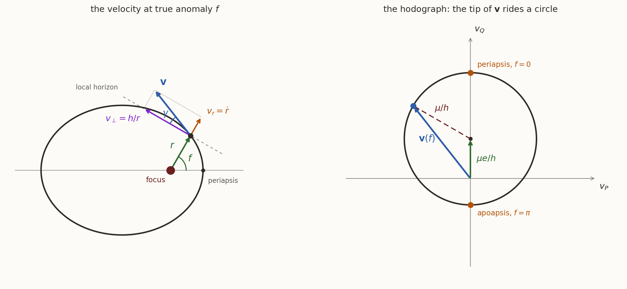
Every Kepler orbit, ellipse, parabola or hyperbola, has a circular hodograph. What differs is where the origin of velocity space sits, and how much of the circle is used.
- \(e<1\): the origin (\(\mu e/h\) from the centre) is inside the circle (radius \(\mu/h\)). The whole circle is traversed, and the velocity points in every direction once per orbit.
- \(e=1\): the origin is on the circle. The speed \(v=0\) is reached, but only in the limit at infinity.
- \(e>1\): the origin is outside the circle. Only an arc is traversed, and the velocity is confined to a wedge of directions.
For \(e>1\), the velocity directions available are those of lines from the origin of velocity space to points of the arc. The extreme directions are along the two tangents from the origin to the circle. What is the half-angle of that wedge? (You will meet this angle again in Section 5.)
Answer
The tangent from a point at distance \(d=\mu e/h\) to a circle of radius \(\rho=\mu/h\) makes an angle \(\alpha\) with the line to the centre, where \(\sin\alpha=\rho/d=1/e\). The two tangent directions are the directions of the velocity at infinity, incoming and outgoing. So the flyby turns the velocity through an angle \(\delta\) with \(\sin(\delta/2)=1/e\); this is the turning angle of Section 5.History: the hodograph. William Rowan Hamilton published the circularity of the hodograph in 1846–47 and used it to give a geometric derivation of the Kepler orbit. Möbius and Maxwell later used it as a teaching device. It is perhaps the cleanest single statement of what is special about the inverse-square law.
2.13.1 Speed and flight path angle on the four conics
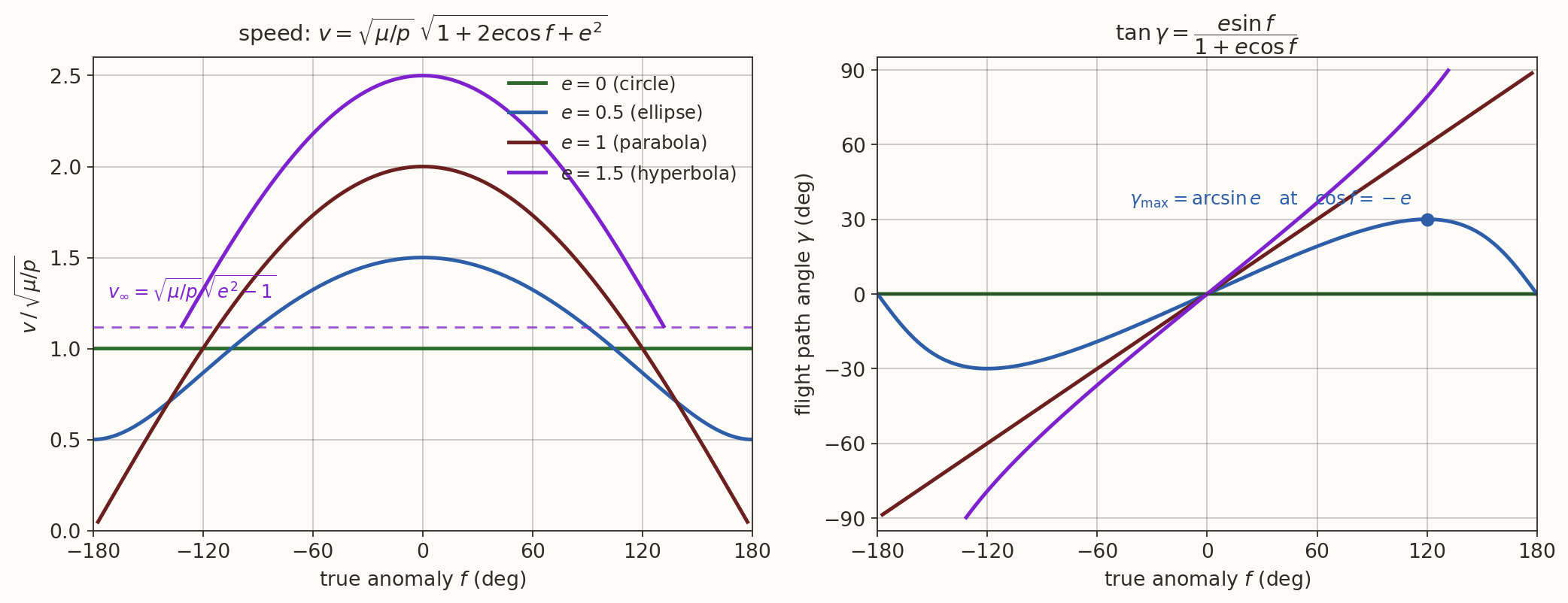
Figure 3 plots Equation 24 and Equation 25 for one orbit of each type.
| orbit | \(e\) | \(v(f)\) | \(\gamma\) | hodograph |
|---|---|---|---|---|
| circle | \(0\) | \(\sqrt{\mu/a}\), constant | \(0\) | circle centred on the origin |
| ellipse | \(0<e<1\) | \(\sqrt{\mu/p}\sqrt{1+2e\cos f+e^2}\) | \(\lvert\gamma\rvert\le\arcsin e\) | origin inside |
| parabola | \(1\) | \(\sqrt{2\mu/r}=2\sqrt{\mu/p}\,\lvert\cos\tfrac f2\rvert\) | \(f/2\) | origin on the circle |
| hyperbola | \(>1\) | \(\sqrt{\mu/p}\sqrt{1+2e\cos f+e^2}\), \(\to v_\infty\) | \(\to\pm90^\circ\) at the asymptotes | origin outside |
For the hyperbola, at \(\cos f_\infty=-1/e\) Equation 24 gives
\[ v_\infty^2=\frac{\mu}{p}\left(1-2+e^2\right)=\frac{\mu}{p}\left(e^2-1\right)=\frac{\mu}{|a|}=C_3 , \]
the characteristic energy of Equation 17, recovered from the velocity side.
2.14 From \(r(f)\) to \(r(t)\)
Everything so far gives the orbit and the velocity as functions of the true anomaly \(f\). None of it says when the body is at a given \(f\). That is the last question, and the hardest.
From Equation 20, \(h=r^2\dot f\), so
\[ dt=\frac{r^2}{h}\,df . \]
Substituting the orbit equation and integrating from periapsis (\(f=0\) at \(t=t_p\), the time of periapsis passage),
\[ t-t_p=\frac{p^2}{h}\int_0^f\frac{df'}{\left(1+e\cos f'\right)^2}. \tag{30}\]
This is the whole problem of timing. The integral is elementary, but it is ugly, and the result cannot be solved for \(f\) as a function of \(t\) in closed form.
Try it on the circle first: set \(e=0\) in Equation 30 and find \(f(t)\). Then try \(e=0.5\) by any means you like (a table of integrals, or a computer algebra system). Can you solve the result for \(f\)?
What you should find
For \(e=0\): \(t-t_p=(p^2/h)f\), so \(f=(h/p^2)(t-t_p)\), uniform motion. For \(e\ne0\) the integral is a combination of \(\arctan\!\left(\sqrt{\tfrac{1-e}{1+e}}\tan\tfrac f2\right)\) and \(\dfrac{\sin f}{1+e\cos f}\), and no algebra will turn “time equals arctan plus a rational function of sines” into “\(f\) equals something”.The classical remedy is not to fight the integral but to change the variable. And this is where the conics finally separate: the substitution that tames \((1+e\cos f)^{-2}\) is different for \(e<1\), \(e=1\) and \(e>1\).
2.15 Where the three conics part ways
Everything up to here holds on every orbit, with no case distinction:
\[ r=\frac{p}{1+e\cos f},\quad h=r^2\dot f,\quad \varepsilon=-\frac{\mu}{2a},\quad v^2=\mu\left(\frac2r-\frac1a\right), \]
\[ v_r=\frac{\mu}{h}e\sin f,\quad v_\perp=\frac{\mu}{h}\left(1+e\cos f\right),\quad \tan\gamma=\frac{e\sin f}{1+e\cos f}. \]
What is left is genuinely different for each conic:
| question | \(e<1\) | \(e=1\) | \(e>1\) |
|---|---|---|---|
| an auxiliary variable that tames Equation 30 | eccentric anomaly \(E\) | \(D=\tan\frac f2\) | hyperbolic anomaly \(H\) |
| the resulting Kepler equation | \(M=E-e\sin E\) | \(M_p=D+\frac{D^3}{3}\) | \(M_h=e\sinh H-H\) |
| can it be inverted in closed form? | no | yes (a cubic) | no |
together with a few quantities that exist only for some conics: the apoapsis \(r_a\) and the period \(T\) (ellipse only), and \(v_\infty\), \(C_3\) and the turning angle (hyperbola only). The next three parts take the conics one at a time; nothing already derived is derived again.
3 The ellipse (\(0\le e<1\))
3.1 What is new
Bound motion. Everything in Section 2 still holds word for word. What the restriction \(e<1\) adds is:
- \(a>0\) becomes a genuine length on the figure, the semi-major axis;
- an apoapsis exists, \(r_a=a(1+e)\), so the curve is closed and encloses a finite area;
- a finite area swept at a constant rate gives a period \(T\);
- the closed curve has an auxiliary circle, and with it the eccentric anomaly \(E\), which tames the time integral.
3.2 Why \(a\) is the semi-major axis
In Section 2.7 we defined \(a\) by \(p=a(1-e^2)\) and claimed nothing about its geometry. For \(e<1\) we can now show that it is exactly half the distance from periapsis to apoapsis.
Put \(f=0\) and \(f=180^\circ\) in the orbit equation. The apoapsis distance is finite only because \(e<1\):
\[ r_p=\frac{p}{1+e},\qquad r_a=\frac{p}{1-e}. \]
The major axis runs from apoapsis to periapsis straight through the focus, so its length is \(r_p+r_a\), and half of it is
\[ \frac{r_p+r_a}{2}=\frac p2\left(\frac1{1+e}+\frac1{1-e}\right)=\frac p2\cdot\frac{(1-e)+(1+e)}{1-e^2}=\frac{p}{1-e^2}=a . \]
So the defined \(a\) and the drawn semi-major axis are the same number, for bound orbits. Three corollaries we use constantly:
\[ r_p=a(1-e),\qquad r_a=a(1+e),\qquad h^2=\mu a\left(1-e^2\right). \tag{31}\]
Given only \(r_p\) and \(r_a\), how do you find \(a\) and \(e\)? Apply it to a transfer orbit from \(300\) km altitude to geostationary radius: \(r_p=6678\) km, \(r_a=42\,164\) km.
Answer
\(a=(r_p+r_a)/2\) and \(e=(r_a-r_p)/(r_a+r_p)\), from adding and subtracting the first two of Equation 31. Here \(a=24\,421\) km and \(e=0.7265\). We will use this orbit, a geostationary transfer orbit (GTO), as a running example.3.3 The period
A closed orbit repeats, and the time per revolution is its period \(T\). We have a quick way to find it: area is swept at a constant rate, so \(T\) is the total area divided by that rate.
Step 1: the rate. In Section 2.2 we found \(dA/dt=h/2\) (Kepler’s second law), using \(h=r^2\dot f\) from Equation 20.
Step 2: the area. An ellipse of semi-axes \(a\) and \(b\) has area \(\pi ab\), so we need the semi-minor axis \(b\). It follows from the orbit equation alone. Put \(\cos f=-e\) in \(r=a(1-e^2)/(1+e\cos f)\):
\[ r=\frac{a\left(1-e^2\right)}{1-e^2}=a,\qquad r\cos f=-ae . \]
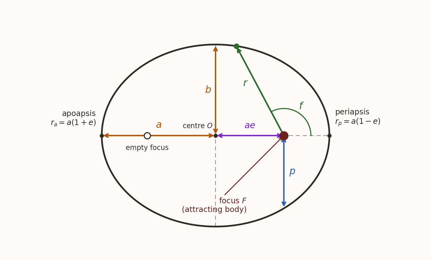
This point lies a distance \(ae\) to the left of the focus (the side away from periapsis). But the centre is also \(ae\) to the left of the focus (Figure 4), so the point sits directly above the centre: it is the end of the minor axis. Its distance from the centre is \(b\) and from the focus is \(a\), so by Pythagoras
\[ b^2=a^2-(ae)^2\qquad\Longrightarrow\qquad b=a\sqrt{1-e^2}=\sqrt{ap}. \tag{32}\]
(This is also the point of steepest climb found in Section 2.12, where \(r=a\).)
Step 3: divide.
\[ T=\frac{\pi ab}{h/2}=\frac{2\pi\,a\cdot a\sqrt{1-e^2}}{\sqrt{\mu a\left(1-e^2\right)}}=\frac{2\pi a^2}{\sqrt{\mu a}}, \]
\[ \boxed{\;T=2\pi\sqrt{\frac{a^3}{\mu}},\qquad n\equiv\frac{2\pi}{T}=\sqrt{\frac{\mu}{a^3}}.\;} \tag{33}\]
The quantity \(n\) is the mean motion, the average angular rate; we need it for Kepler’s equation.
Once again \(e\) has cancelled: the period, like the energy, depends only on \(a\). Indeed \(T\) and \(\varepsilon=-\mu/2a\) are two readings of the same number. This is Kepler’s third law, with the constant now explained: \(T^2/a^3=4\pi^2/\mu\).
History: Newton’s correction to Kepler’s third law. Kepler stated \(T^2\propto a^3\) with the same constant for every planet. Newton’s version, \(T^2=4\pi^2a^3/(G(m_1+m_2))\), shows that the constant depends on the planet’s mass too. For Jupiter, the heaviest planet, \(T^2/a^3\) is smaller than for a massless planet by the factor \(1/(1+1/1047)=0.99905\), a part in a thousand. Kepler’s data could not show this, and neither can the four-figure table in the \(N\)-body note.
Two period calculations. (a) Find the period of the space station’s orbit (\(r=6791\) km). (b) A geostationary satellite must complete one revolution per sidereal day, \(86\,164.1\) s, the Earth’s rotation period relative to the stars. Find the radius of its circular orbit.
What you should find
\(T=2\pi\sqrt{6791^3/398\,600}=5569\) s \(=92.8\) min, about \(15.5\) orbits a day.
\(a=\left(\mu\,(T/2\pi)^2\right)^{1/3}=42\,164\) km, i.e. \(35\,786\) km above the equator.
In the explorer of Section 2.10, drive with \(a\) and sweep \(e\). Does the period change?
Answer
No. \(T\) depends on \(a\) alone. A circle of radius \(a\) and a needle-thin ellipse of semi-major axis \(a\) take exactly the same time to go round.3.4 Two bodies in three dimensions: an example
Here is a full example that uses most of what we have so far. Take units with \(G=1\) and two equal masses, \(m_1=m_2=\tfrac12\), so \(\mu=G(m_1+m_2)=1\). At \(t=0\):
\[ \begin{aligned} \mathbf R_1(0)&=\left(+\tfrac12,0,0\right),&\qquad \mathbf V_1(0)&=\tfrac12\,\hat{\mathbf y},\\ \mathbf R_2(0)&=\left(-\tfrac12,0,0\right),&\qquad \mathbf V_2(0)&=\tfrac12\,\hat{\mathbf z}. \end{aligned} \]
The bodies sit on the \(x\)-axis; one is launched along \(y\), the other along \(z\). Before reading on, try to predict the motion.
Work out the orbit from the initial data alone. (a) Find the relative state \(\mathbf r(0)=\mathbf R_2-\mathbf R_1\) and \(\dot{\mathbf r}(0)=\mathbf V_2-\mathbf V_1\). (b) From it compute \(\mathbf h\), \(\varepsilon\), then \(a\), \(e\) and \(T\), without integrating anything. (c) Is the starting point periapsis, apoapsis, or neither?
What you should find
\(\mathbf r(0)=-\hat{\mathbf x}\) and \(\dot{\mathbf r}(0)=\tfrac12(\hat{\mathbf z}-\hat{\mathbf y})\).
\(\mathbf h=\mathbf r\times\dot{\mathbf r}=\tfrac12(\hat{\mathbf y}+\hat{\mathbf z})\), so \(h=1/\sqrt2\). \(\varepsilon=v^2/2-\mu/r=\tfrac14-1=-\tfrac34\). Then \(a=-\mu/2\varepsilon=\tfrac23\), \(e=\sqrt{1+2\varepsilon h^2/\mu^2}=\sqrt{1-\tfrac34}=\tfrac12\) and \(T=2\pi\sqrt{a^3/\mu}=3.4201\).
\(\mathbf r\cdot\dot{\mathbf r}=0\), so \(\dot r=0\) and the start is an apsis. Since \(r(0)=1=a(1+e)\), it is the apoapsis.
There is one more feature of this initial state. The total momentum is \(\mathbf P=m_1\mathbf V_1+m_2\mathbf V_2=\tfrac14(\hat{\mathbf y}+\hat{\mathbf z})\ne\mathbf 0\), so the barycentre drifts, at \(\mathbf V_{\rm cm}=\mathbf P/M=\tfrac14(\hat{\mathbf y}+\hat{\mathbf z})\). This is parallel to \(\mathbf h\): the barycentre moves along the normal to the orbital plane. The plane of the relative orbit is carried through space face-first, like a sheet pushed along its normal, and neither body ever returns to a point it has visited. In the inertial frame each body traces a helix, even though the relative orbit is a closed ellipse of period \(3.4201\) (Figure 5).
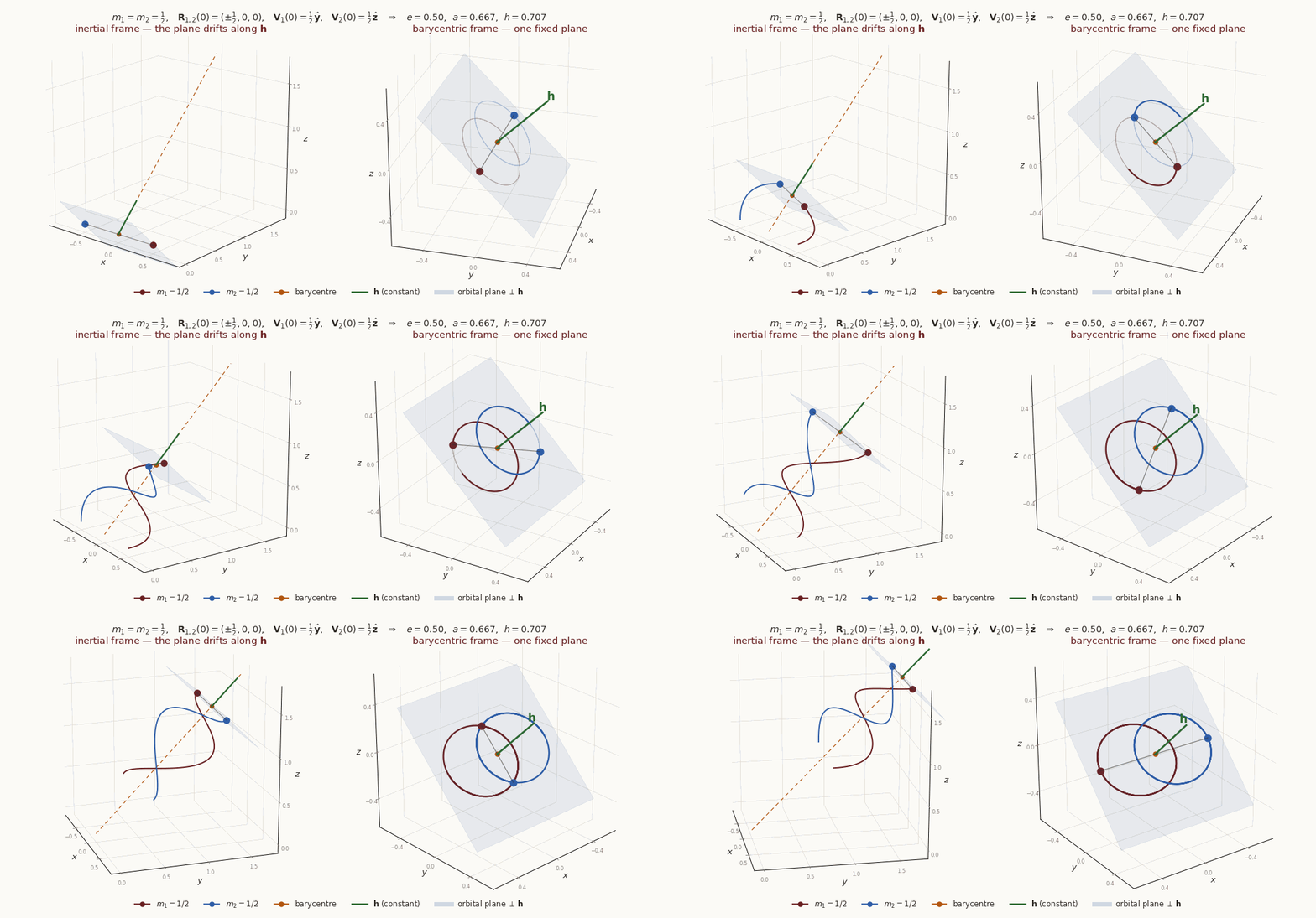
What must be true of the initial data for both bodies to move in a single fixed plane in the inertial frame as well?
Answer
In the barycentric frame both bodies lie in the plane through the barycentre perpendicular to \(\mathbf h\) (by Equation 2, both are multiples of \(\mathbf r\)). In the inertial frame that plane is carried along by \(\mathbf V_{\rm cm}t\). It stays the same plane only if the drift lies in it: \(\mathbf V_{\rm cm}\cdot\mathbf h=0\), i.e. \((m_1\mathbf V_1+m_2\mathbf V_2)\cdot(\mathbf r\times\dot{\mathbf r})=0\) at \(t=0\). Here the drift is along \(\mathbf h\), the worst case.3.5 Speed and direction on an ellipse
3.5.1 Scaling out the size
Divide the velocity components Equation 22, Equation 21 and the speed Equation 24 by \(\sqrt{\mu/a}\), the circular speed at radius \(a\). With \(\mu/h=\sqrt{\mu/p}=\sqrt{\mu/a}/\sqrt{1-e^2}\),
\[ \frac{v_r}{\sqrt{\mu/a}}=\frac{e\sin f}{\sqrt{1-e^2}},\qquad \frac{v_\perp}{\sqrt{\mu/a}}=\frac{1+e\cos f}{\sqrt{1-e^2}}, \]
\[ \frac{v}{\sqrt{\mu/a}}=\frac{\sqrt{1+2e\cos f+e^2}}{\sqrt{1-e^2}}. \]
The semi-major axis has disappeared: \(e\) fixes the shape of all three curves, and \(a\) only sets the scale.
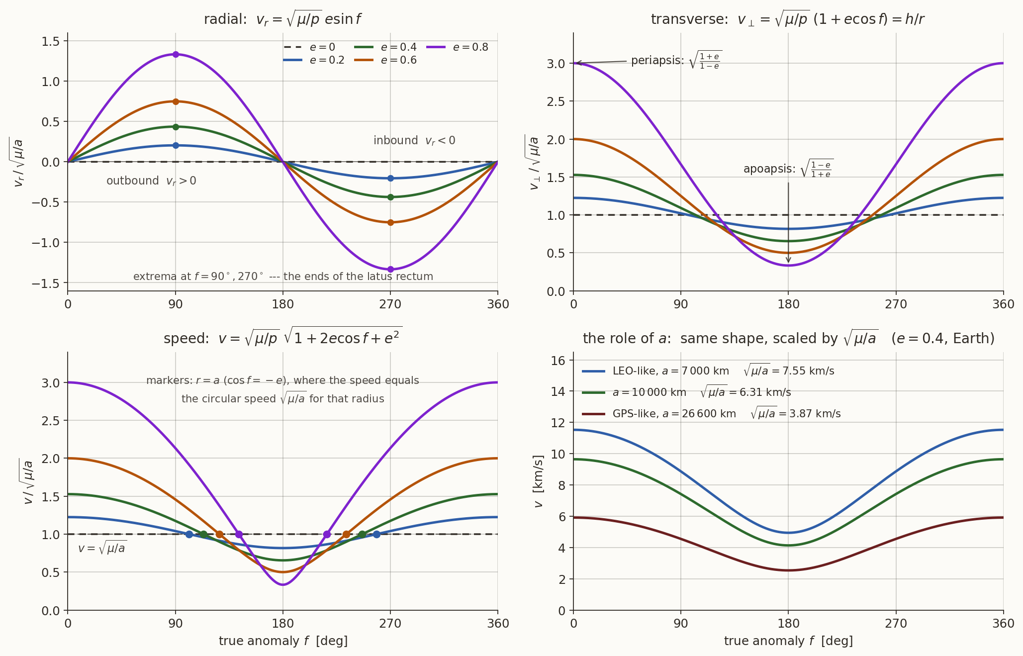
What the figure shows:
- \(v_r\) is odd about the line of apsides. It vanishes at both apsides and is largest in size at \(f=\pm90^\circ\), where \(|v_r|=(\mu/h)e\). Outbound is positive, inbound negative.
- \(v_\perp\) never changes sign. It is \(h/r\), largest at periapsis and smallest at apoapsis.
- The speed equals \(\sqrt{\mu/a}\) exactly where \(r=a\), at \(\cos f=-e\) (the ends of the minor axis). Vis-viva says so at once: \(v^2=\mu(2/r-1/a)=\mu/a\) when \(r=a\). Inside that radius the body is faster than its “average” speed \(\sqrt{\mu/a}\); outside, slower.
- Eccentric orbits are lopsided in time as well as speed. The body hurries through periapsis and dawdles at apoapsis, which is Kepler’s second law seen from the velocity side.
3.5.2 Apsidal speeds
Put \(f=0\) and \(f=180^\circ\) in Equation 24:
\[ \begin{aligned} v_p&=\sqrt{\frac{\mu}{p}}(1+e)=\sqrt{\frac{\mu}{a}\,\frac{1+e}{1-e}},\\[2pt] v_a&=\sqrt{\frac{\mu}{p}}(1-e)=\sqrt{\frac{\mu}{a}\,\frac{1-e}{1+e}}. \end{aligned} \tag{34}\]
From Equation 34 find \(v_p/v_a\) and \(v_pv_a\). Interpret both.
What you should find
\[ \frac{v_p}{v_a}=\frac{1+e}{1-e}=\frac{r_a}{r_p},\qquad v_pv_a=\frac{\mu}{p}\left(1-e^2\right)=\frac{\mu}{a}. \]
The first is \(h=rv\) at the two apsides (the velocity is perpendicular to \(\mathbf r\) there, so \(h=r_pv_p=r_av_a\)). The second says that the geometric mean of the two apsidal speeds is the circular speed at radius \(a\).3.5.3 The flight path angle across a family of ellipses
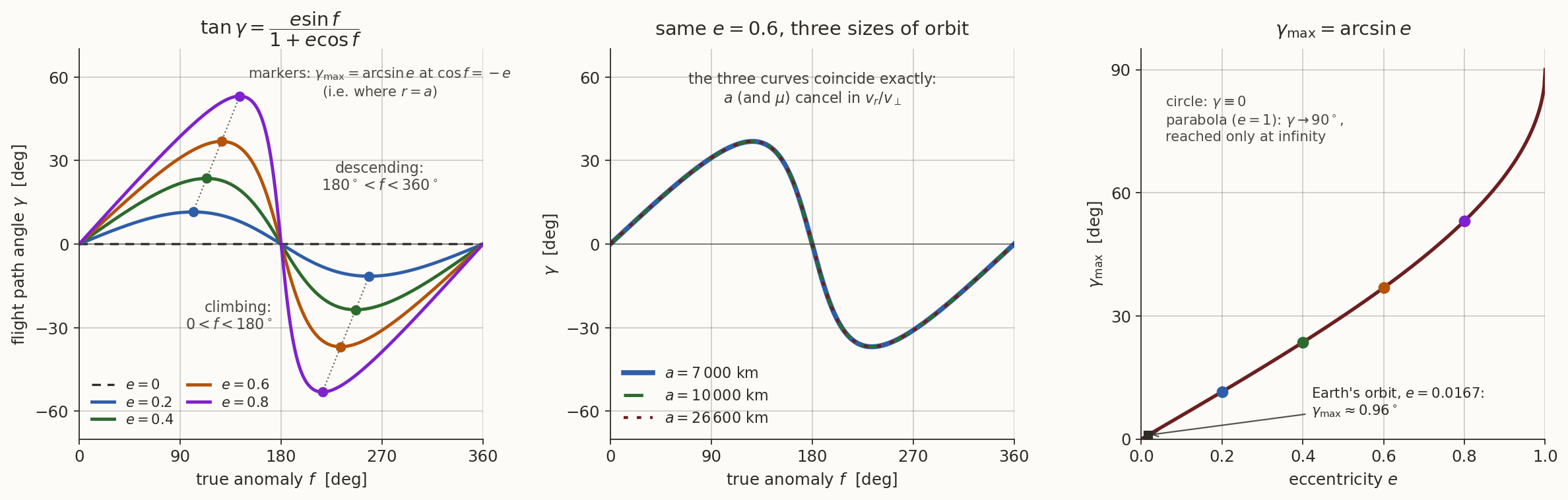
Figure 7 confirms what Equation 25 said: \(a\) does nothing to \(\gamma\); \(e\) does everything. \(\gamma_{\max}=\arcsin e\) grows slowly at first (\(e=0.2\) gives \(11.5^\circ\)) and then quickly (\(e=0.8\) gives \(53^\circ\)), approaching \(90^\circ\) as \(e\to1\).
The flight path angle is easy to draw with the wrong sign. Figure 8 draws it at one point in each quadrant of an ellipse.
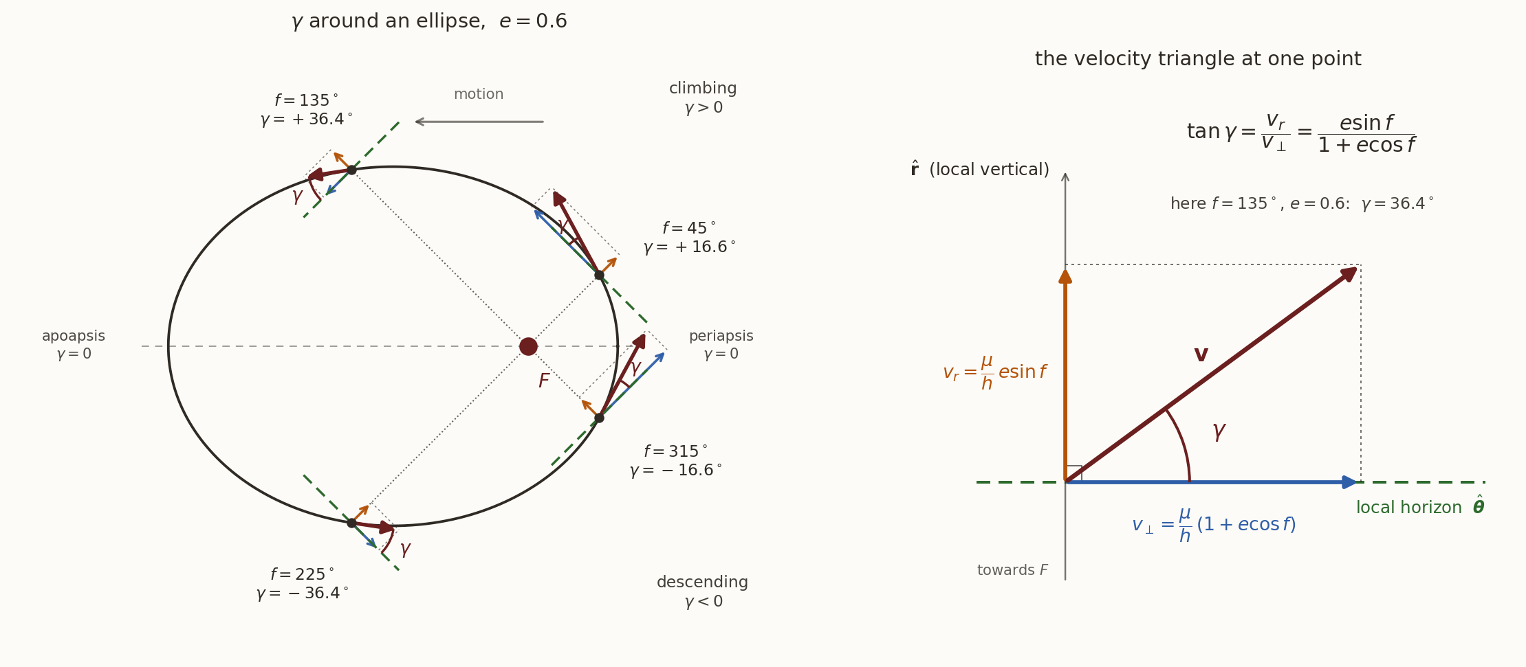
Look at Figure 8. (a) Why is the “horizontal” in the figure not horizontal on the page? (b) Which arrow keeps its sense all the way round, and which reverses? (c) The figure gives \(\gamma=16.6^\circ\) at \(f=45^\circ\) and \(36.4^\circ\) at \(f=135^\circ\). What are the values at \(f=315^\circ\) and \(f=225^\circ\)?
Answer
The local horizontal is perpendicular to \(\mathbf r\), so it turns with the body. \(\gamma\) is measured from a reference that itself rotates.
The blue \(v_\perp=h/r\) always points the same way round the orbit; it carries all of the angular momentum. The amber \(v_r\) reverses between the second and third quadrants, and that reversal is the sign of \(\gamma\): climbing on the way out, descending on the way back.
\(-16.6^\circ\) and \(-36.4^\circ\): same radius, same speed, velocity reflected in the line of apsides. (With \(e=0.6\) the steepest climb is \(\arcsin0.6=36.87^\circ\) at \(f=126.87^\circ\), so the \(135^\circ\) point is within half a degree of it.)
An orbit is raised by a small burn \(\delta v\) applied along the velocity at periapsis. Show that the periapsis distance does not change, and find how much the apoapsis distance changes. Where does the energy go?
Answer
After a burn along the velocity at periapsis, the velocity is still perpendicular to \(\mathbf r\) there, so the burn point is still an apsis of the new orbit, and since the speed went up it is still the periapsis: \(\delta r_p=0\). All of the change happens on the far side. The energy changes by \(\delta\varepsilon=v_p\,\delta v\) (to first order), and from \(\varepsilon=-\mu/2a\), \(\delta a=(2a^2/\mu)\,\delta\varepsilon\). With \(r_a=2a-r_p\),
\[ \delta r_a=2\,\delta a=\frac{4a^2v_p}{\mu}\,\delta v . \]
For a circular orbit \(400\) km up, \(4a^2v_p/\mu\approx3500\) km per km/s: each metre per second raises the far side by about \(3.5\) km. The energy goes into potential energy on the far side. The lever arm \(4a^2v_p/\mu\) grows with \(v_p\), which is why burns are most effective where the speed is high (the Oberth effect).3.5.4 Worked example: a geostationary transfer orbit
Take the GTO of the earlier Check box: \(r_p=6678\) km, \(r_a=42\,164\) km, so \(a=24\,421\) km and \(e=0.7265\), with \(\mu=398\,600\) km\(^3\)/s\(^2\).
Compute the perigee and apogee speeds, check \(v_p/v_a=r_a/r_p\), and find where the climb is steepest: the true anomaly, \(\gamma\), the radius and the speed there.
What you should find
From Equation 34, \(v_p=10.15\) km/s and \(v_a=1.608\) km/s; \(v_p/v_a=6.31=r_a/r_p\). The steepest climb is at \(\cos f=-e\), i.e. \(f=136.6^\circ\), where \(\gamma=\arcsin0.7265=46.6^\circ\), \(r=a=24\,421\) km and \(v=\sqrt{\mu/a}=4.04\) km/s.
The spacecraft starts at \(10.15\) km/s and arrives at geostationary height at only \(1.61\) km/s, whereas a geostationary satellite moves at \(3.07\) km/s. The difference is what the apogee engine has to supply.At which true anomaly is a body on an ellipse moving at exactly the local circular speed \(\sqrt{\mu/r}\)? Is it a coincidence that this is also where \(\gamma\) is largest?
Answer
Vis-viva gives \(\mu(2/r-1/a)=\mu/r\), i.e. \(r=a\), i.e. \(1+e\cos f=p/a=1-e^2\), so \(\cos f=-e\): the ends of the minor axis. Not a coincidence. From Equation 26, \(\gamma\) is stationary exactly where \(\cos f=-e\). Both are the single fact \(r=a\): inside that radius the body is faster than a circular orbit there, outside it is slower, and at the crossing its velocity leans furthest from the horizontal.3.6 The eccentric anomaly and Kepler’s equation
We return to the timing problem Equation 30. For the ellipse the trick is geometric: describe the position not by the angle \(f\) at the focus, but by an angle at the centre of the ellipse.
3.6.1 The auxiliary circle
Draw the auxiliary circle, of radius \(a\), centred at the centre \(O\) of the ellipse (Figure 9). From the body \(P\), drop a perpendicular to the major axis and extend it to meet the circle at \(Q\). The eccentric anomaly \(E\) is the angle at the centre from the direction of periapsis to \(Q\).
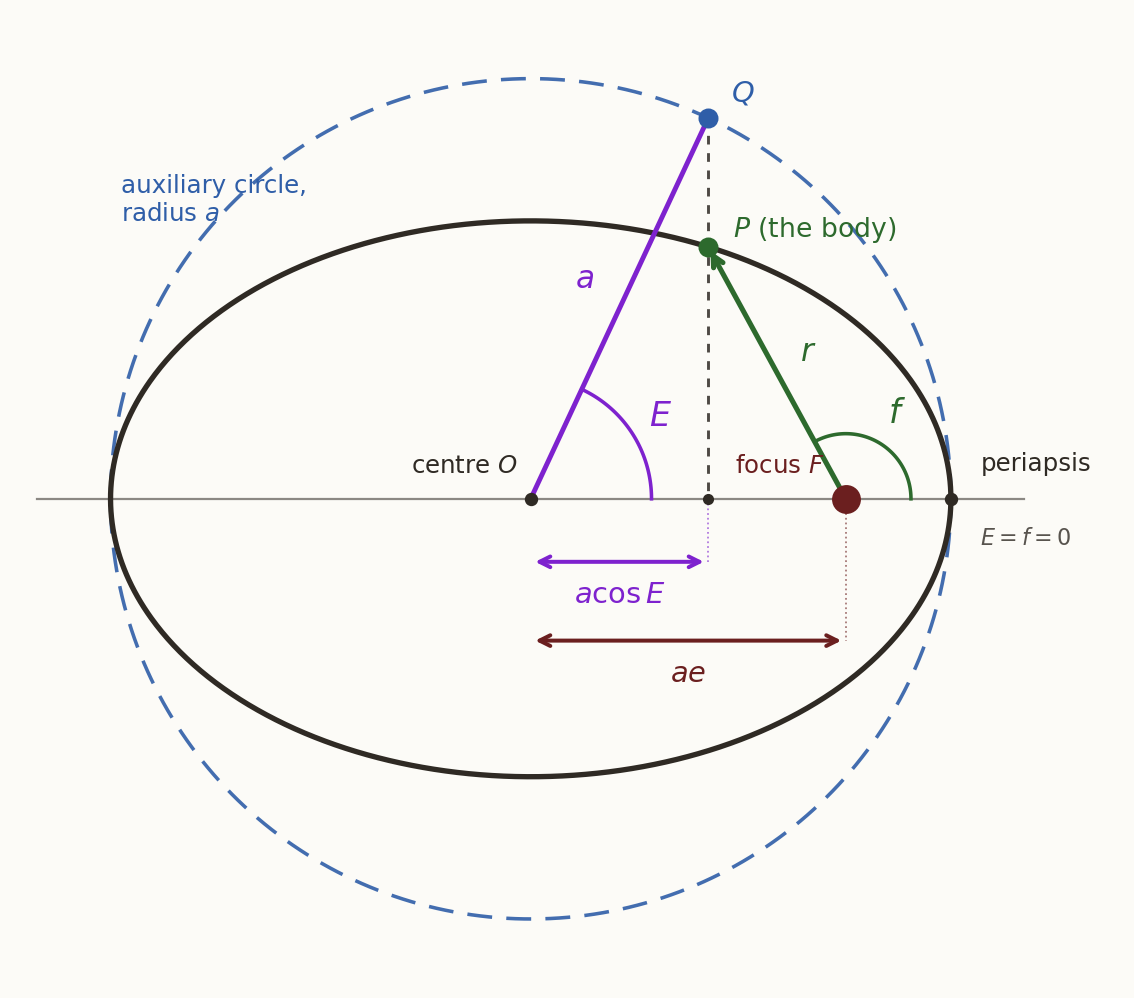
With the origin at \(O\) and the \(x\)-axis towards periapsis, \(Q=(a\cos E,\ a\sin E)\), and by construction \(x_P=x_Q=a\cos E\). To find \(y_P\) use the equation of the ellipse about its centre:
\[ \frac{x_P^2}{a^2}+\frac{y_P^2}{b^2}=1 \quad\xrightarrow{\;x_P=a\cos E\;}\quad y_P^2=b^2\left(1-\cos^2E\right)=b^2\sin^2E, \]
so \(P=(a\cos E,\ b\sin E)\): the ellipse is the auxiliary circle squashed vertically by \(b/a\). The focus is at \((ae,0)\) relative to \(O\), so measured from the focus,
\[ x=a\left(\cos E-e\right),\qquad y=b\sin E=a\sqrt{1-e^2}\,\sin E . \tag{35}\]
Now compute the distance from the focus:
\[ \begin{aligned} r^2=x^2+y^2&=a^2\left(\cos E-e\right)^2+a^2\left(1-e^2\right)\sin^2E\\ &=a^2\left[\cos^2E-2e\cos E+e^2+\sin^2E-e^2\sin^2E\right]\\ &=a^2\left[1-2e\cos E+e^2\cos^2E\right]=a^2\left(1-e\cos E\right)^2, \end{aligned} \]
\[ \boxed{\;r=a\left(1-e\cos E\right).\;} \tag{36}\]
Compare with \(r=a(1-e^2)/(1+e\cos f)\): the radius is now linear in \(\cos E\) instead of reciprocal in \(\cos f\). That is the first sign that \(E\) is the better variable.
Check Equation 36 at \(E=0\) and \(E=180^\circ\). Why are these the natural points to check?
Answer
\(E=0\) gives \(a(1-e)=r_p\) and \(E=180^\circ\) gives \(a(1+e)=r_a\). They are the natural checks because the apsides are the only points where \(E\) and \(f\) agree: both are measured from the direction of periapsis, and on the major axis the vertical projection from the ellipse to the circle does nothing.3.6.2 Taming the time integral
We need \(\int r^2\,df\). In polar coordinates about the focus, \(x=r\cos f\) and \(y=r\sin f\), and a short calculation (try it) shows that
\[ x\,dy-y\,dx=r^2\,df . \]
So we can compute \(r^2df\) from Equation 35, with \(dx=-a\sin E\,dE\) and \(dy=a\sqrt{1-e^2}\cos E\,dE\):
\[ \begin{aligned} r^2\,df&=a\left(\cos E-e\right)\cdot a\sqrt{1-e^2}\cos E\,dE\\ &\qquad-a\sqrt{1-e^2}\sin E\cdot\left(-a\sin E\,dE\right)\\ &=a^2\sqrt{1-e^2}\left[\cos^2E-e\cos E+\sin^2E\right]dE\\ &=a^2\sqrt{1-e^2}\left(1-e\cos E\right)dE . \end{aligned} \]
The awkward \((1+e\cos f)^{-2}\) has become a linear factor. Using \(h=\sqrt{\mu a(1-e^2)}\),
\[ dt=\frac{r^2\,df}{h}=\frac{a^2\sqrt{1-e^2}}{\sqrt{\mu a}\sqrt{1-e^2}}\left(1-e\cos E\right)dE=\sqrt{\frac{a^3}{\mu}}\left(1-e\cos E\right)dE . \]
Integrating from periapsis (\(E=0\) at \(t=t_p\)),
\[ t-t_p=\sqrt{\frac{a^3}{\mu}}\left(E-e\sin E\right). \]
The prefactor is \(1/n\), with \(n\) the mean motion of Equation 33. Defining the mean anomaly
\[ \boxed{\;M\equiv n\left(t-t_p\right)=\frac{2\pi}{T}\left(t-t_p\right),\;} \tag{37}\]
the result is Kepler’s equation:
\[ \boxed{\;M=E-e\sin E.\;} \tag{38}\]
Two quick checks: \(e=0\) gives \(M=E=f\) (a circle, swept uniformly); and \(E=2\pi\) gives \(M=2\pi\), so \(t-t_p=T\), one full revolution.
What \(M\) is. Of the three anomalies, \(M\) is the only one that is not an angle you can point at on the figure. It is the angle of a fictitious body that goes round a circle of radius \(a\) at the constant rate \(n\), passing periapsis together with the real one. Equivalently, by Kepler’s second law, it is the swept area turned into an angle: \(M=2\pi\times(\text{area swept since periapsis})/(\pi ab)\).
| anomaly | symbol | measured at | how it changes with time |
|---|---|---|---|
| true | \(f\) | the focus | the physical angle; non-uniform |
| eccentric | \(E\) | the centre | a computational intermediary |
| mean | \(M\) | (nowhere) | linear in \(t\), by construction |
3.6.3 Relating \(E\) and \(f\)
To use Kepler’s equation we must convert between \(E\) and \(f\). From Equation 35 and Equation 36, the polar coordinates of the body about the focus give
\[ \cos f=\frac xr=\frac{\cos E-e}{1-e\cos E},\qquad\sin f=\frac yr=\frac{\sqrt{1-e^2}\sin E}{1-e\cos E}. \tag{39}\]
A single formula, valid in every quadrant, is better. Use \(\tan\frac f2=\dfrac{\sin f}{1+\cos f}\). The denominator is
\[ 1+\cos f=1+\frac{\cos E-e}{1-e\cos E}=\frac{(1-e)(1+\cos E)}{1-e\cos E}, \tag{40}\]
so
\[ \tan\frac f2=\frac{\sqrt{1-e^2}\sin E}{(1-e)(1+\cos E)}=\sqrt{\frac{1+e}{1-e}}\,\frac{\sin E}{1+\cos E}, \]
and since \(\sin E/(1+\cos E)=\tan\frac E2\),
\[ \boxed{\;\tan\frac f2=\sqrt{\frac{1+e}{1-e}}\,\tan\frac E2.\;} \tag{41}\]
\(\frac f2\) and \(\frac E2\) are always in the same quadrant, so this never confuses quadrants (in a program, use the two-argument arctangent near \(E=180^\circ\), where both tangents blow up).
3.6.4 Solving Kepler’s equation
The three anomalies give the standard way to find the position at time \(t\), given \(a\), \(e\) and \(t_p\):
\[ t\;\longrightarrow\;M=n(t-t_p)\;\longrightarrow\;E\;\longrightarrow\;f\;\longrightarrow\;r,\ \mathbf v . \]
- \(t\to M\) is trivial; that is the whole point of \(M\).
- \(M\to E\) is the hard step. Equation 38 is transcendental: it has no solution in elementary functions. The standard tool is Newton’s method. With \(g(E)=E-e\sin E-M\),
\[ E_{k+1}=E_k-\frac{E_k-e\sin E_k-M}{1-e\cos E_k}, \tag{42}\]
started from \(E_0=M\) (or \(E_0=\pi\) when \(e\) is close to \(1\)). The denominator is \(1-e\cos E=r/a>0\), so the iteration is well defined for every \(e<1\), and near the root it converges quadratically. - \(E\to f\) uses Equation 41. - \(\to r\): in fact \(r=a(1-e\cos E)\) needs no \(f\) at all; \(f\) is needed only to orient \(\mathbf r\) in the plane, and for the velocity.
Solve \(M=E-e\sin E\) for \(e=0.5\) and \(M=1\) rad by Newton’s method from \(E_0=1\). Keep nine decimals. How many correct digits do you gain per step? Then find \(f\) and \(r/a\).
What you should find
\(E_1=1.576469353\), \(E_2=1.500208269\), \(E_3=1.498701721\), \(E_4=1.498701134\). The error goes roughly \(5\times10^{-1}\to8\times10^{-2}\to2\times10^{-3}\to6\times10^{-7}\to10^{-13}\): the number of correct digits roughly doubles each step (quadratic convergence). Then \(f=116.36^\circ\) from Equation 41, and \(r/a=1-0.5\cos E=0.964\).The sixth constant. Rather than \(t_p\), catalogues usually quote the mean anomaly at epoch, \(M_0=n(t_0-t_p)\), at a stated epoch \(t_0\); then \(M(t)=M_0+n(t-t_0)\). It is the same information, but it stays well defined as \(e\to0\), where periapsis, and hence \(t_p\), ceases to exist. This is the timing constant promised in Section 2.6: five constants fix the curve, and \(M_0\) fixes where on it the body is.
History: Kepler’s problem. Kepler met this equation in Astronomia Nova (1609) and could not solve it. He wrote that he was satisfied it could not be solved a priori, because the arc and the sine are quantities of different kinds, and promised that whoever showed him how would be “the great Apollonius” to him.
He was right: \(E(M)\) is not an elementary function. Expanding \(E\) in powers of \(e\) (Lagrange’s series) converges only for \(e<0.6627\), the Laplace limit. Bessel’s expansion in the functions now named after him, \(E=M+\sum_{k\ge1}\frac2k\,J_k(ke)\sin kM\), converges for every \(e<1\); Bessel introduced these functions for this very problem. Hundreds of papers on solving Kepler’s equation have appeared since.
3.6.5 How the three anomalies are related
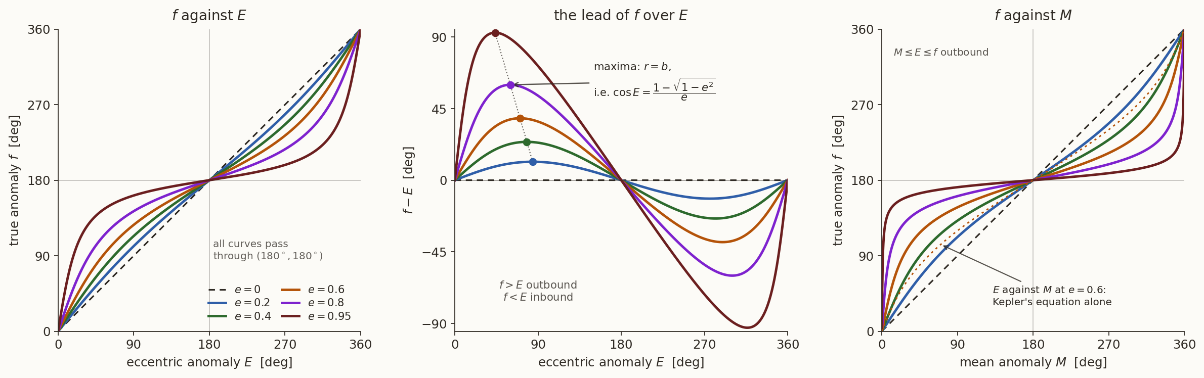
The left and right panels of Figure 10 look alike, but they answer different questions. \(E\leftrightarrow f\) is about a picture: freeze the ellipse, and the two angles describe the same point seen from two places, the centre and the focus. No clock is involved. \(M\leftrightarrow f\) is about time: \(M\) is Kepler’s second law turned into an angle.
Why the curves bend. Differentiate Equation 41:
\[ \tfrac12\sec^2\tfrac f2\,df=\sqrt{\frac{1+e}{1-e}}\;\tfrac12\sec^2\tfrac E2\,dE , \]
so
\[ \frac{df}{dE}=\sqrt{\frac{1+e}{1-e}}\,\frac{\cos^2\frac f2}{\cos^2\frac E2}=\sqrt{\frac{1+e}{1-e}}\,\frac{1+\cos f}{1+\cos E}. \]
Using Equation 40 for \(1+\cos f\),
\[ \frac{df}{dE}=\sqrt{\frac{1+e}{1-e}}\,\frac{1-e}{1-e\cos E}=\frac{\sqrt{1-e^2}}{1-e\cos E}=\frac{b/a}{r/a} \qquad\Longrightarrow\qquad \boxed{\;\frac{df}{dE}=\frac br.\;} \]
That one formula reads off the whole left panel:
- \(r<b\) (near periapsis): \(f\) runs ahead of \(E\). The focus is close to periapsis, so a small displacement there subtends a large angle at the focus but a smaller one at the centre.
- \(r>b\) (near apoapsis): \(f\) falls behind \(E\).
- \(r=b\): they run level, and the lead \(f-E\) is largest (centre panel).
- \(E=0\) and \(180^\circ\) are fixed points for every \(e\): there the centre, the focus and the body are in line.
For \(M\), differentiate Kepler’s equation and use the chain rule:
\[ \frac{dM}{dE}=1-e\cos E=\frac ra, \qquad \frac{dM}{df}=\frac{dM}{dE}\,\frac{dE}{df}=\frac ra\cdot\frac rb , \]
\[ \boxed{\;\frac{dM}{df}=\frac{r^2}{ab}.\;} \]
This is not a new fact: it is Kepler’s second law in another form, since \(dA=\tfrac12r^2df\) and \(M=2A/(ab)\). Each pair of anomalies runs level at its own radius:
| relation | derivative | runs level where |
|---|---|---|
| \(M\) against \(E\) | \(dM/dE=r/a\) | \(r=a\) |
| \(f\) against \(E\) | \(df/dE=b/r\) | \(r=b\) |
| \(f\) against \(M\) | \(df/dM=ab/r^2\) | \(r=\sqrt{ab}\) |
and since \(b\le\sqrt{ab}\le a\), the three crossings occur in that order as the body climbs from periapsis. On the outbound half, \(M\le E\le f\): the real body runs ahead of its fictitious uniformly moving twin after periapsis, because that is where it is fastest.
For nearly circular orbits, show that
\[ \begin{aligned} f&=E+e\sin E+O(e^2),\\ E&=M+e\sin M+O(e^2),\\ \text{hence}\quad f&=M+2e\sin M+O(e^2). \end{aligned} \]
How far ahead of its mean position does the Earth (\(e=0.0167\)) get?
Answer
From \(df/dE=\sqrt{1-e^2}/(1-e\cos E)=1+e\cos E+O(e^2)\), integrating from \(0\) gives \(f=E+e\sin E+O(e^2)\). From Kepler’s equation \(E=M+e\sin E\), and replacing \(E\) by \(M\) inside the sine costs only \(O(e^2)\), so \(E=M+e\sin M+O(e^2)\). Adding the two leads, \(f=M+2e\sin M+O(e^2)\).
For the Earth, the largest lead is \(2e=0.0334\) rad \(=1.9^\circ\). The Sun’s apparent position in the sky runs up to about \(1.9^\circ\) ahead of or behind its average position. Since the Sun moves about \(1^\circ\) per day, that is almost two days, and it is a major part of the equation of time (the difference between sundial time and clock time).3.6.6 Worked example: propagating an eccentric geosynchronous orbit
Not every geosynchronous orbit is geostationary. Take an eccentric, Tundra-type orbit: the period is one sidereal day, but the orbit is far from circular. With \(\mu=398\,600.4\) km\(^3\)/s\(^2\),
\[ a=42\,164~\text{km},\quad e=0.25, \]
so that \(r_p=31\,623\) km, \(r_a=52\,705\) km, \(b=40\,825\) km, and
\[ n=\sqrt{\frac{\mu}{a^3}}=7.29216\times10^{-5}~\text{rad/s},\qquad T=\frac{2\pi}{n}=86\,163.6~\text{s}=23^{\rm h}56^{\rm m}04^{\rm s}. \]
At \(t_0\) the spacecraft is at \(f_0=30^\circ\). Where is it six hours later?
Before reading the solution, plan it: which way round the pipeline must you go first?
Step 0: run the pipeline backwards to find the clock. We are given \(f_0\), not \(M_0\), so first \(f\to E\to M\):
\[ \tan\frac{E_0}{2}=\sqrt{\frac{1-e}{1+e}}\,\tan\frac{f_0}{2}=\sqrt{\frac{0.75}{1.25}}\tan15^\circ , \]
so \(E_0=23.4508^\circ=0.409294\) rad, and
\[ M_0=E_0-e\sin E_0=0.409294-0.25\sin(0.409294)=0.309804~\text{rad}, \]
i.e. \(M_0=17.7504^\circ\).
So \(t_0-t_p=M_0/n=4248.5\) s \(=1.180\) h: the spacecraft passed perigee \(1.18\) hours earlier. Its radius is \(r_0=a(1-e\cos E_0)=32\,494\) km.
Step 1: \(t\to M\). Six hours is \(21\,600\) s:
\[ M_1=M_0+n\,\Delta t=0.309804+1.575107=1.884910~\text{rad}=107.997^\circ . \]
Step 2: \(M\to E\). Newton’s method on \(g(E)=E-e\sin E-M_1\), from \(E=M_1\):
| \(k\) | \(E_k\) (rad) | \(g(E_k)\) | \(\Delta E_k\) |
|---|---|---|---|
| 0 | \(1.884910\) | \(-2.378\times10^{-1}\) | \(+2.207\times10^{-1}\) |
| 1 | \(2.105629\) | \(+5.630\times10^{-3}\) | \(-4.994\times10^{-3}\) |
| 2 | \(2.100635\) | \(+2.685\times10^{-6}\) | \(-2.383\times10^{-6}\) |
| 3 | \(2.100633\) | \(+6.1\times10^{-13}\) | — |
\(E_1=2.100633\) rad \(=120.3574^\circ\). The residual goes \(10^{-1}\to10^{-3}\to10^{-6}\to10^{-13}\), the signature of quadratic convergence. The derivative \(1-e\cos E=r/a\) was about \(1.13\), far from zero: a well-conditioned problem.
Step 3: \(E\to f\).
\[ \tan\frac{f_1}{2}=\sqrt{\frac{1.25}{0.75}}\tan(60.179^\circ)\quad\Longrightarrow\quad f_1=132.118^\circ . \]
Step 4: the state. Two independent routes to \(r\) must agree:
\[ \begin{aligned} r_1&=a\left(1-e\cos E_1\right)=47\,491~\text{km},\\ r_1&=\frac{p}{1+e\cos f_1}=\frac{39\,529~\text{km}}{1+0.25\cos132.118^\circ}=47\,491~\text{km}.\ \checkmark \end{aligned} \]
Then \(v_1=\sqrt{\mu(2/r_1-1/a)}=2.708\) km/s and, from Equation 25, \(\gamma_1=12.56^\circ\): still climbing towards apogee.
Read the three anomalies at the final instant, \(M_1=108.00^\circ\), \(E_1=120.36^\circ\) and \(f_1=132.12^\circ\). Is their order what you expect? Explain the \(24^\circ\) difference between \(f_1\) and \(M_1\) in one sentence.
Answer
Yes: on the outbound half, \(M\le E\le f\). The spacecraft is \(24^\circ\) ahead of its fictitious uniformly moving twin because it has just spent seven hours near perigee, where it moves fastest.4 The parabola (\(e=1\))
4.1 The one-parameter conic
Set \(e=1\) in the orbit equation and use \(1+\cos f=2\cos^2\frac f2\):
\[ r=\frac{p}{1+\cos f}=\frac p2\sec^2\frac f2,\qquad r_p=\frac p2\quad(f=0). \]
There is no second parameter. An ellipse needs two numbers for its size and shape, \((a,e)\); a parabola is fixed by one, \(p\), or equivalently \(r_p\) or \(h=\sqrt{\mu p}\). Its eccentricity is not a free number but the defining condition.
The formulas of Section 2 specialise by putting \(e=1\):
\[ \varepsilon=\frac{\mu\left(e^2-1\right)}{2p}=0,\qquad a=\frac{p}{1-e^2}\to\infty . \]
So never use \(a\) for a parabola. Vis-viva becomes
\[ \boxed{\;v^2=\frac{2\mu}{r},\;} \]
the escape speed of Equation 16: a body on a parabola moves at exactly the local escape speed at every point. It reaches infinity, and arrives there with nothing left.
4.2 Speed and direction on a parabola
Put \(e=1\) in the speed Equation 24 and the flight path angle Equation 25, and simplify with half-angle formulas. What is \(\gamma\) as a function of \(f\)?
What you should find
\[ v=\sqrt{\frac{\mu}{p}}\sqrt{2+2\cos f}=2\sqrt{\frac{\mu}{p}}\left|\cos\frac f2\right|, \]
\[ \tan\gamma=\frac{\sin f}{1+\cos f}=\frac{2\sin\frac f2\cos\frac f2}{2\cos^2\frac f2}=\tan\frac f2, \]
so \(\boxed{\gamma=f/2}\). The speed agrees with \(\sqrt{2\mu/r}\), as it must.The result \(\gamma=f/2\) says that the direction of motion turns at exactly half the rate of the position vector. As \(f\) runs from \(-180^\circ\) to \(180^\circ\), \(\gamma\) runs from \(-90^\circ\) to \(90^\circ\): the velocity swings through half a turn, from radially inbound at infinity to radially outbound at infinity. The hodograph is still the circle of radius \(\mu/h\), but now the origin of velocity space lies on it: \(v=0\) is reached, once, at infinity.
Why are there no parabolic orbits in nature?
Answer
\(\varepsilon=0\) is a single value in a continuum: initial conditions with exactly zero energy are infinitely improbable, and any disturbance (a third body, outgassing, radiation pressure) moves \(\varepsilon\) off zero. Long-period comets arrive on orbits with \(e=0.999\ldots\), ellipses with periods of hundreds of thousands of years or more. Astronomers often fit them as parabolas because the short arc observed near perihelion cannot distinguish \(e=1\) from \(e=1\pm10^{-3}\).
The parabola matters because it is the boundary between capture and escape. “Escape” means crossing it.4.3 Time on a parabola: Barker’s equation
The time integral Equation 30 with \(e=1\) is
\[ t-t_p=\frac{p^2}{h}\int_0^f\frac{df'}{\left(1+\cos f'\right)^2}=\frac{p^2}{4h}\int_0^f\sec^4\frac{f'}{2}\,df' . \]
Here the right substitution is suggested by the integrand itself: \(\sec^4\) is \(\sec^2\times\sec^2\), one \(\sec^2\) is the derivative of \(\tan\), and the other is \(1+\tan^2\). So put
\[ D=\tan\frac f2,\qquad dD=\tfrac12\sec^2\frac f2\,df,\qquad\sec^2\frac f2=1+D^2 . \]
\(D\) is the parabolic anomaly. Like \(E\), it is not an angle you can point at, but it turns the integrand into something simple:
\[ \frac{p^2}{4h}\sec^4\frac f2\,df=\frac{p^2}{4h}\left(1+D^2\right)\cdot2\,dD=\frac{p^2}{2h}\left(1+D^2\right)dD . \]
The integral is now a polynomial. With \(h=\sqrt{\mu p}\) and \(p=2r_p\),
\[ t-t_p=\frac{p^2}{2h}\left(D+\frac{D^3}{3}\right)=\sqrt{\frac{2r_p^3}{\mu}}\left(D+\frac{D^3}{3}\right). \]
Defining the parabolic mean anomaly \(M_p\equiv\sqrt{\mu/(2r_p^3)}\,(t-t_p)\),
\[ \boxed{\;M_p=D+\frac{D^3}{3},\qquad D=\tan\frac f2 .\;} \tag{43}\]
This is Barker’s equation.
History: Barker’s equation. It is named after Thomas Barker, who in 1757 published tables for the motion of comets on parabolic orbits based on it. Comets were the main application: in the eighteenth and nineteenth centuries most newly discovered comets were fitted with parabolic orbits first.
Unlike Kepler’s equation, Equation 43 is a cubic in \(D\), so it can be inverted in closed form. Since \(dM_p/dD=1+D^2>0\), \(M_p\) increases strictly with \(D\) and there is exactly one real root. Writing \(D^3+3D-3M_p=0\), Cardano’s formula gives
\[ D=\sqrt[3]{\frac{3M_p}{2}+\sqrt{\frac{9M_p^2}{4}+1}}+\sqrt[3]{\frac{3M_p}{2}-\sqrt{\frac{9M_p^2}{4}+1}}, \tag{44}\]
and then \(f=2\arctan D\).
Apart from the trivial circle, the parabola is the only conic whose timing problem has an elementary solution.
A comet moves on a parabola with perihelion at \(r_p=0.5\) AU (\(\mu_\odot=1.327\times10^{11}\) km\(^3\)/s\(^2\), \(1~\text{AU}=1.496\times10^{8}\) km).
- How long does it take to go from perihelion out to the Earth’s distance, \(1\) AU? (Find \(f\) from the orbit equation first.) (b) Where is it \(20\) days after perihelion? Use Equation 44. (c) How fast is it moving when it crosses the Earth’s orbit?
What you should find
\(p=2r_p=1\) AU, so \(r=1\) AU needs \(1+\cos f=1\), \(f=90^\circ\), \(D=1\) and \(M_p=4/3\). With \(\sqrt{2r_p^3/\mu}=2.512\times10^{6}\) s, \(t-t_p=3.35\times10^{6}\) s \(=38.8\) days.
\(M_p=20\times86\,400/2.512\times10^{6}=0.688\), and Equation 44 gives \(D=0.612\), so \(f=62.9^\circ\) and \(r=p/(1+\cos f)=0.687\) AU.
\(\sqrt{2\mu_\odot/1~\text{AU}}=42.1\) km/s, the local escape speed from the Sun. Compare the Earth’s \(29.8\) km/s.
5 The hyperbola (\(e>1\))
Hyperbolic orbits are the orbits of spacecraft leaving a planet for another, and of spacecraft flying past a planet. Two questions dominate: how fast is the spacecraft when it is far away, and how much does the planet bend its path?
5.1 Geometry
With \(e>1\), Equation 10 gives a negative \(a\). Writing \(|a|=p/(e^2-1)\), every formula reads naturally:
\[ r=\frac{|a|\left(e^2-1\right)}{1+e\cos f},\qquad r_p=\frac{p}{1+e}=|a|(e-1), \]
\[ \varepsilon=-\frac{\mu}{2a}=+\frac{\mu}{2|a|}>0 . \]
The body exists only on \(|f|<f_\infty\), with \(\cos f_\infty=-1/e\) (Equation 6). Geometrically (Figure 11):
- \(|a|\) is the distance from the centre of the hyperbola to its vertex (periapsis). The focus is a further \(|a|e\) from the centre, so \(r_p=|a|e-|a|=|a|(e-1)\).
- The asymptotes make the angle \(\arccos(1/e)\) with the line of apsides, measured at the centre.
- The other branch of the hyperbola is the path a body would follow under a repulsive inverse-square force with the same \(h\) and \(\varepsilon\). It is not physical here.
Vis-viva is best written with the sign of \(a\) made explicit:
\[ \boxed{\;v^2=\mu\left(\frac2r+\frac1{|a|}\right),\;} \tag{45}\]
larger than the local escape speed \(\sqrt{2\mu/r}\) everywhere, by a margin that does not vanish as \(r\to\infty\).
5.2 Speed at infinity
Letting \(r\to\infty\) in Equation 45,
\[ \boxed{\;v_\infty=\sqrt{\frac{\mu}{|a|}}=\sqrt{2\varepsilon},\qquad C_3=v_\infty^2=\frac{\mu}{|a|}=-\frac{\mu}{a}.\;} \]
For a departing interplanetary spacecraft, \(v_\infty\) is the only thing that survives to interplanetary distances: it is the spacecraft’s velocity relative to the planet once it has left the planet’s neighbourhood.
5.3 Turning angle
The body arrives along the asymptote \(f=-f_\infty\) and leaves along \(f=+f_\infty\). The direction of motion therefore turns through the turning angle
\[ \delta=2f_\infty-\pi . \]
(At infinity the velocity is along the asymptote, i.e. radial; its direction changes from \(-f_\infty+\pi\) on arrival to \(+f_\infty\) on departure.) Then \(\sin\frac\delta2=\sin\left(f_\infty-\frac\pi2\right)=-\cos f_\infty\), and with Equation 6,
\[ \boxed{\;\sin\frac\delta2=\frac1e .\;} \tag{46}\]
This is the angle you found from the hodograph in Section 2.13. Combining \(r_p=|a|(e-1)\) with \(|a|=\mu/v_\infty^2\) expresses \(e\) through the two quantities a mission designer controls:
\[ \boxed{\;e=1+\frac{r_pv_\infty^2}{\mu}.\;} \tag{47}\]
So a flyby is steered by how deep the spacecraft goes and how fast it arrives. Slow and deep turns hard (\(e\to1\), \(\delta\to180^\circ\)); fast and shallow barely bends (\(e\to\infty\), \(\delta\to0\)).
A spacecraft passes Jupiter (\(\mu=1.267\times10^{8}\) km\(^3\)/s\(^2\)) with \(v_\infty=6\) km/s and periapsis radius \(r_p=10^{6}\) km. Through what angle is it turned? Does its speed relative to Jupiter change?
Answer
\(e=1+10^{6}\times36/(1.267\times10^{8})=1.284\) and \(\delta=2\arcsin(1/1.284)=102.3^\circ\).
Relative to Jupiter the speed does not change: \(v_\infty\) in equals \(v_\infty\) out, by energy conservation. Only the direction changes, by more than a right angle. But relative to the Sun, that rotated \(\mathbf v_\infty\) is added to Jupiter’s own orbital velocity of \(13.1\) km/s, so the spacecraft’s speed about the Sun can change by up to \(2v_\infty\sin(\delta/2)\) (here \(9.3\) km/s). That is a gravity assist; the momentum comes from Jupiter, whose orbit changes by an immeasurably small amount.5.4 The aiming radius, and what \(b\) means for a hyperbola
The perpendicular distance from the focus to the incoming asymptote is the aiming radius (or impact parameter) \(\Delta\). It is the distance by which the spacecraft would miss the planet if gravity were switched off. At infinity the lever arm of the velocity about the focus is \(\Delta\), so
\[ h=\Delta\,v_\infty . \]
For the ellipse, \(b\) was a length we could measure: the semi-minor axis, from the centre to the curve. A hyperbola never crosses the perpendicular to the line of apsides through its centre (it needs \(|x|\ge|a|\) there), so for \(e>1\) the symbol \(b\) must be defined. Eliminating \(f\) from the orbit equation and moving the origin to the centre gives
\[ \frac{x^2}{|a|^2}-\frac{y^2}{b^2}=1,\qquad b^2\equiv c^2-|a|^2=|a|^2\left(e^2-1\right), \]
where \(c=|a|e\) is the centre-to-focus distance (for the ellipse, \(b^2=a^2-c^2\); the two terms have swapped). Three equivalent ways to see this number:
- Asymptote slope. The asymptotes are \(y=\pm(b/|a|)x\), the diagonals of the rectangle \(|x|\le|a|\), \(|y|\le b\).
- The same \(p\) relation as the ellipse: \(b^2=|a|p\).
- The distance from the focus to an asymptote is exactly \(b\). So the aiming radius is \(\Delta=b=|a|\sqrt{e^2-1}\).
Check that \(h=\Delta v_\infty\) agrees with \(h^2=\mu p\), using \(\Delta=|a|\sqrt{e^2-1}\), \(v_\infty^2=\mu/|a|\) and \(p=|a|(e^2-1)\).
What you should find
\(\Delta^2v_\infty^2=|a|^2(e^2-1)\cdot\mu/|a|=\mu|a|(e^2-1)=\mu p=h^2\). \(\checkmark\)Note that \(b\) is larger than \(|a|\) when \(e>\sqrt2\), so “semi-minor axis” is a misnomer for a hyperbola. Figure 11 is drawn at \(e=1.6\), where \(b>|a|\).
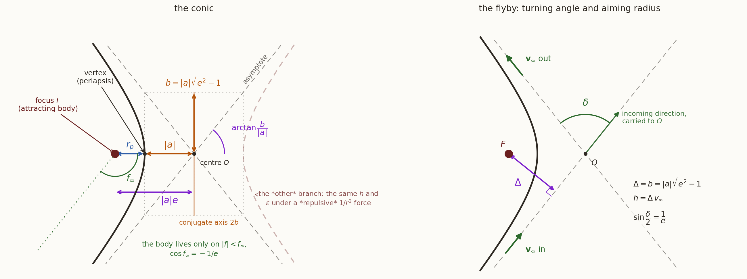
5.5 The hyperbolic anomaly \(H\)
For timing we copy the elliptic trick. There, the auxiliary curve was a circle and \(x=a(\cos E-e)\). For the hyperbola the auxiliary curve is a rectangular hyperbola, and the circular functions become hyperbolic functions, \(\cosh H=\frac12(e^H+e^{-H})\) and \(\sinh H=\frac12(e^H-e^{-H})\), which satisfy \(\cosh^2H-\sinh^2H=1\) (Figure 12). Measured from the focus,
\[ x=|a|\left(e-\cosh H\right),\qquad y=|a|\sqrt{e^2-1}\,\sinh H . \tag{48}\]
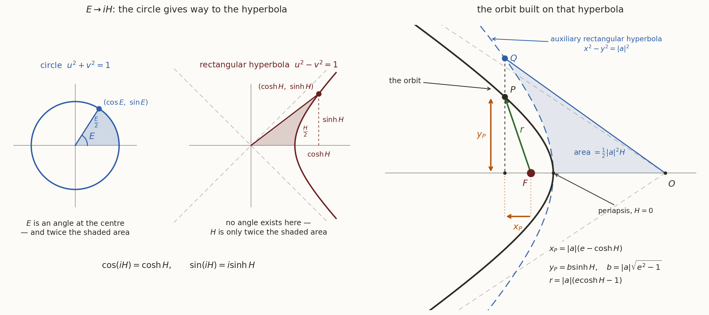
Repeat the calculation that led to Equation 36, with Equation 48, to show that \(r=|a|(e\cosh H-1)\). You need only \(\cosh^2H-\sinh^2H=1\).
What you should find
\[ \begin{aligned} r^2&=a^2\left(e-\cosh H\right)^2+a^2\left(e^2-1\right)\sinh^2H\\ &=a^2\left[e^2-2e\cosh H+\cosh^2H+\left(e^2-1\right)\left(\cosh^2H-1\right)\right]\\ &=a^2\left[e^2\cosh^2H-2e\cosh H+1\right]=a^2\left(e\cosh H-1\right)^2 . \end{aligned} \]So
\[ \boxed{\;r=|a|\left(e\cosh H-1\right),\;} \tag{49}\]
the elliptic \(r=a(1-e\cos E)\) with \(\cos\to\cosh\) and the sign flipped, and again linear in the new variable. \(H\) runs over \((-\infty,\infty)\), with \(H=0\) at periapsis and \(H\to\pm\infty\) at the asymptotes. The same half-angle manipulation as for the ellipse gives
\[ \boxed{\;\tanh\frac H2=\sqrt{\frac{e-1}{e+1}}\,\tan\frac f2 .\;} \tag{50}\]
\(\tanh\) never exceeds \(1\), and the right-hand side reaches \(1\) exactly when \(\tan\frac{f_\infty}{2}=\sqrt{(e+1)/(e-1)}\), the asymptote: the whole infinite range of \(H\) is squeezed into the finite window \(|f|<f_\infty\).
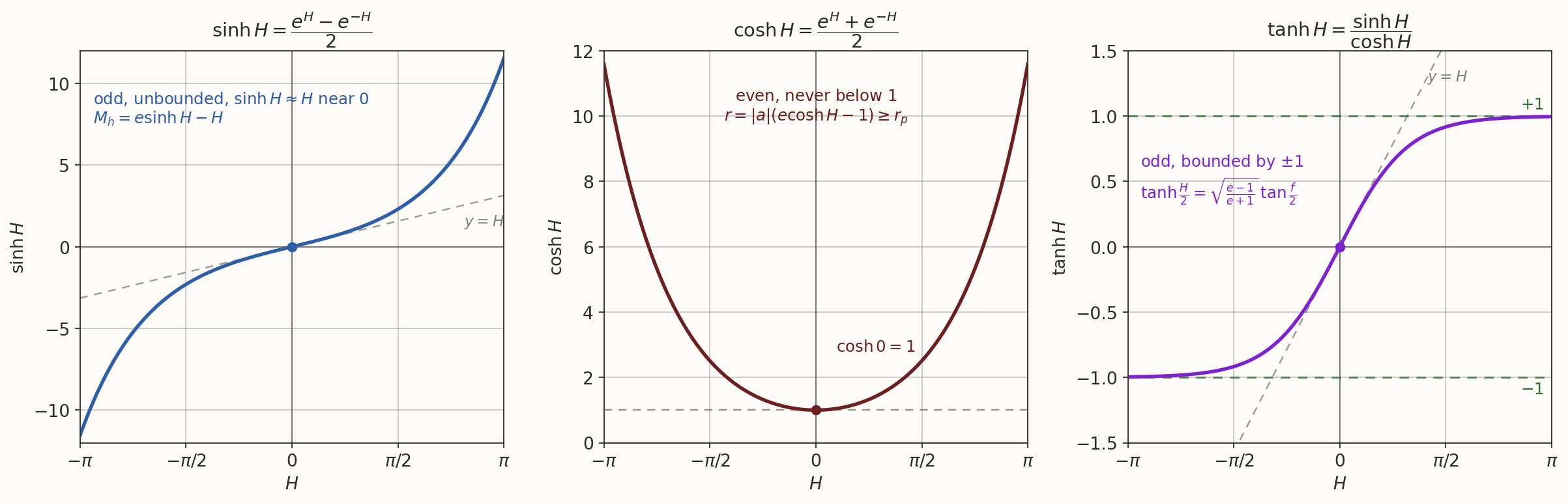
5.6 The hyperbolic Kepler equation
From Equation 48, with \(dx=-|a|\sinh H\,dH\) and \(dy=|a|\sqrt{e^2-1}\cosh H\,dH\),
\[ \begin{aligned} r^2\,df=x\,dy-y\,dx&=|a|^2\sqrt{e^2-1}\left[\left(e-\cosh H\right)\cosh H+\sinh^2H\right]dH\\ &=|a|^2\sqrt{e^2-1}\left(e\cosh H-1\right)dH . \end{aligned} \]
With \(h=\sqrt{\mu|a|(e^2-1)}\),
\[ dt=\frac{r^2\,df}{h}=\sqrt{\frac{|a|^3}{\mu}}\left(e\cosh H-1\right)dH . \]
Integrating from periapsis (\(H=0\) at \(t=t_p\)) and defining
\[ n_h=\sqrt{\frac{\mu}{|a|^3}},\qquad M_h=n_h\left(t-t_p\right), \]
we get the hyperbolic Kepler equation
\[ \boxed{\;M_h=e\sinh H-H .\;} \tag{51}\]
Side by side with its elliptic twin:
| ellipse | hyperbola | |
|---|---|---|
| radius | \(r=a(1-e\cos E)\) | \(r=\lvert a\rvert(e\cosh H-1)\) |
| Kepler equation | \(M=E-e\sin E\) | \(M_h=e\sinh H-H\) |
| derivative | \(dM/dE=1-e\cos E=r/a\) | \(dM_h/dH=e\cosh H-1=r/\lvert a\rvert\) |
| range | \(E\in[0,2\pi)\), periodic | \(H\in(-\infty,\infty)\), never repeats |
Both derivatives equal \(r/|a|>0\), so both equations have exactly one root, and Newton’s method,
\[ H_{k+1}=H_k-\frac{e\sinh H_k-H_k-M_h}{e\cosh H_k-1}, \]
is well defined. The practical difference is the starting guess: \(\sinh\) grows exponentially, so \(H_0=M_h\) is poor for large \(M_h\); a common choice is \(H_0=\ln\left(2M_h/e+1.8\right)\). There is no period and no repetition: everything about a hyperbolic pass happens once.
A spacecraft leaves a \(300\) km parking orbit (\(r_p=6678\) km) on a hyperbola with \(v_\infty=3\) km/s. How long does it take to reach \(925\,000\) km, roughly the edge of the Earth’s sphere of influence? Plan: find \(|a|\) and \(e\); get \(H\) from Equation 49; get \(M_h\) from Equation 51; divide by \(n_h\). (Here no iteration is needed: we know \(r\) and want \(t\).)
What you should find
\(|a|=\mu/v_\infty^2=44\,289\) km and \(e=1+r_pv_\infty^2/\mu=1.1506\). At \(r=925\,000\) km, \(\cosh H=(r/|a|+1)/e=19.02\), so \(H=3.638\) and \(M_h=1.1506\sinh(3.638)-3.638=18.22\). With \(n_h=\sqrt{\mu/|a|^3}=6.77\times10^{-5}\) s\(^{-1}\), \(t-t_p=2.69\times10^{5}\) s \(=3.11\) days.
For comparison, the periapsis speed is \(\sqrt{v_\infty^2+2\mu/r_p}=11.34\) km/s, and the turning angle of this hyperbola is \(2\arcsin(1/1.1506)=120.7^\circ\).6 The conics side by side
| circle | ellipse | parabola | hyperbola | |
|---|---|---|---|---|
| \(e\) | \(0\) | \(0<e<1\) | \(1\) | \(>1\) |
| \(\varepsilon\) | \(<0\) | \(<0\) | \(0\) | \(>0\) |
| \(a=p/(1-e^2)\) | \(a=r\) | \(a>0\) | \(\to\infty\) | \(a<0\) |
| range of \(f\) | all | all | \(\lvert f\rvert<180^\circ\) | \(\lvert f\rvert<\arccos(-1/e)\) |
| \(r_p\) | \(a\) | \(a(1-e)\) | \(p/2\) | \(\lvert a\rvert(e-1)\) |
| \(r_a\) | \(a\) | \(a(1+e)\) | — | — |
| period | \(2\pi\sqrt{a^3/\mu}\) | \(2\pi\sqrt{a^3/\mu}\) | — | — |
| speed at \(\infty\) | — | — | \(0\) | \(\sqrt{\mu/\lvert a\rvert}\) |
| largest \(\lvert\gamma\rvert\) | \(0\) | \(\arcsin e\) | \(90^\circ\) (limit) | \(90^\circ\) (limit) |
| auxiliary variable | \(f\) itself | \(E\) | \(D=\tan\frac f2\) | \(H\) |
| Kepler equation | \(M=f\) | \(M=E-e\sin E\) | \(M_p=D+\frac{D^3}{3}\) | \(M_h=e\sinh H-H\) |
| closed-form inverse | trivial | no | yes (cubic) | no |
| hodograph origin | centre | inside | on the circle | outside |
The first nine rows are specialisations of formulas from Section 2. The last four are genuinely separate work for each conic.
Three formulas are worth committing to memory because they never need a case distinction:
\[ r=\frac{p}{1+e\cos f},\qquad v=\sqrt{\frac{\mu}{p}}\sqrt{1+2e\cos f+e^2},\qquad\tan\gamma=\frac{e\sin f}{1+e\cos f}. \]
Given \((p,e,f)\) they return the position, speed and direction on any conic whatsoever.
7 Appendix: the rotating basis
The velocity derivation of Section 2.11 rested on two formulas,
\[ \dot{\hat{\mathbf r}}=\dot f\,\hat{\boldsymbol\theta},\qquad\dot{\hat{\boldsymbol\theta}}=-\dot f\,\hat{\mathbf r}. \]
We prove them twice, once with components and once without.
Setup. Let \(\hat{\mathbf P}\) point from the focus towards periapsis and \(\hat{\mathbf Q}=\hat{\mathbf h}\times\hat{\mathbf P}\) complete a right-handed pair in the orbital plane (the perifocal basis). Both are built from the constants \(\mathbf e\) and \(\mathbf h\), so both are fixed in space. Since \(f\) is measured from periapsis,
\[ \hat{\mathbf r}=\cos f\,\hat{\mathbf P}+\sin f\,\hat{\mathbf Q},\qquad \hat{\boldsymbol\theta}=-\sin f\,\hat{\mathbf P}+\cos f\,\hat{\mathbf Q}. \]
Proof 1: differentiate the components. Only \(f\) depends on time:
\[ \dot{\hat{\mathbf r}}=\dot f\left(-\sin f\,\hat{\mathbf P}+\cos f\,\hat{\mathbf Q}\right)=\dot f\,\hat{\boldsymbol\theta}, \qquad \dot{\hat{\boldsymbol\theta}}=\dot f\left(-\cos f\,\hat{\mathbf P}-\sin f\,\hat{\mathbf Q}\right)=-\dot f\,\hat{\mathbf r}. \]
That is the whole proof, but it hides why it is true.
Proof 2: the unit circle. Two facts suffice.
- The derivative of a unit vector is perpendicular to it. Differentiating \(\hat{\mathbf u}\cdot\hat{\mathbf u}=1\) gives \(2\hat{\mathbf u}\cdot\dot{\hat{\mathbf u}}=0\). A unit vector can only turn; it cannot stretch.
- It turns at the rate of the angle. In a short time the tip of \(\hat{\mathbf r}\) moves along the unit circle by a chord of length \(|\Delta\hat{\mathbf r}|=2\sin(\Delta f/2)\to\Delta f\), and the chord’s direction tends to the tangent, which is \(\hat{\boldsymbol\theta}\).
Dividing by \(\Delta t\) gives \(\dot{\hat{\mathbf r}}=\dot f\,\hat{\boldsymbol\theta}\). The same argument for \(\hat{\boldsymbol\theta}\), whose tip moves towards \(-\hat{\mathbf r}\), gives the second formula.
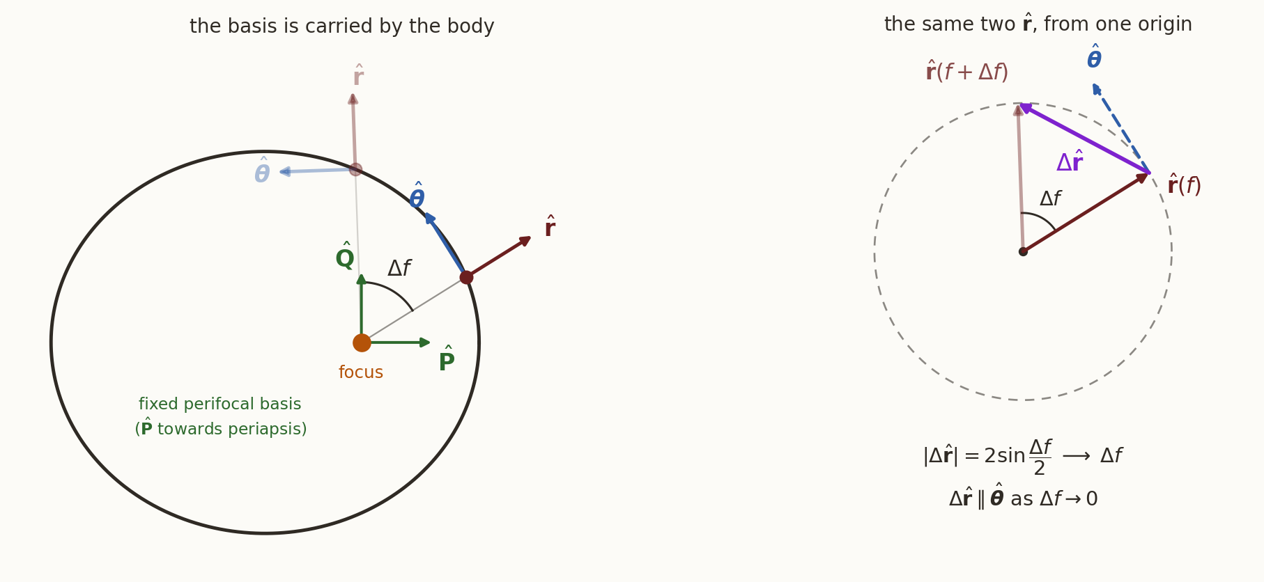
Both formulas as one statement. The pair turns about \(\hat{\mathbf h}\) with angular velocity \(\boldsymbol\omega=\dot f\,\hat{\mathbf h}\), and any vector fixed in a rotating frame changes at the rate \(\boldsymbol\omega\times(\cdot)\). With the right-handed triad \(\hat{\mathbf r}\times\hat{\boldsymbol\theta}=\hat{\mathbf h}\),
\[ \boldsymbol\omega\times\hat{\mathbf r}=\dot f\,\hat{\mathbf h}\times\hat{\mathbf r}=\dot f\,\hat{\boldsymbol\theta}, \qquad \boldsymbol\omega\times\hat{\boldsymbol\theta}=\dot f\,\hat{\mathbf h}\times\hat{\boldsymbol\theta}=-\dot f\,\hat{\mathbf r}. \]
This is the same rule that produces the Coriolis and centrifugal terms in a rotating frame; here the frame’s spin rate \(\dot f=h/r^2\) is handed to us by a conservation law.
7.0.1 The payoff: the equation of motion in polar form
Differentiate \(\mathbf v=\dot r\,\hat{\mathbf r}+r\dot f\,\hat{\boldsymbol\theta}\) once more, using the two formulas at every step:
\[ \ddot{\mathbf r}=\left(\ddot r-r\dot f^2\right)\hat{\mathbf r}+\left(r\ddot f+2\dot r\dot f\right)\hat{\boldsymbol\theta}. \]
Equating to \(-\mu\hat{\mathbf r}/r^2\) splits Equation 1 into two scalar equations:
\[ \ddot r-r\dot f^2=-\frac{\mu}{r^2},\qquad r\ddot f+2\dot r\dot f=\frac1r\frac{d}{dt}\left(r^2\dot f\right)=0 . \]
The transverse equation is the conservation of angular momentum, \(r^2\dot f=h\), found again. Substituting it into the radial equation leaves one equation for \(r(t)\):
\[ \ddot r-\frac{h^2}{r^3}=-\frac{\mu}{r^2}. \tag{52}\]
Derive the orbit equation a second way, from Equation 52. Put \(u=1/r\) and use \(f\) instead of \(t\) as the independent variable (\(\frac{d}{dt}=\frac{h}{r^2}\frac{d}{df}=hu^2\frac{d}{df}\)). Show that \(\dot r=-h\,du/df\) and \(\ddot r=-h^2u^2\,d^2u/df^2\), and hence that Equation 52 becomes
\[ \frac{d^2u}{df^2}+u=\frac{\mu}{h^2}. \]
Solve it. (This is the Binet route; it works for any central force, with \(\mu u^2\) replaced by the force law.)
What you should find
\(\dot r=\frac{d}{dt}(1/u)=-\frac{1}{u^2}hu^2\frac{du}{df}=-h\frac{du}{df}\), and differentiating again, \(\ddot r=-h\,hu^2\frac{d^2u}{df^2}\). Substituting into Equation 52 and dividing by \(-h^2u^2\) gives the equation above: a harmonic oscillator with a constant forcing. Its general solution is \(u=\mu/h^2+C\cos(f-\omega)\); choosing the origin of \(f\) at periapsis (\(\omega=0\)) and writing \(C=e\mu/h^2\),
\[ u=\frac{\mu}{h^2}\left(1+e\cos f\right)\quad\Longleftrightarrow\quad r=\frac{p}{1+e\cos f}. \]
The same conic, with \(e\) now appearing as a constant of integration of an ODE rather than as the length of a conserved vector.8 Summary
- The relative motion of two bodies obeys \(\ddot{\mathbf r}=-\mu\mathbf r/r^3\), \(\mu=G(m_1+m_2)\); the individual motions follow from Equation 2.
- Three integrals: \(\mathbf h=\mathbf r\times\dot{\mathbf r}\) (the motion is planar, and sweeps equal areas in equal times), \(\mathbf e\) (points to periapsis; the orbit does not precess) and \(\varepsilon=v^2/2-\mu/r\). Two Casimir relations leave five independent constants; the sixth is a time, \(t_p\) or \(M_0\).
- The orbit is a conic, \(r=p/(1+e\cos f)\) with \(p=h^2/\mu\). The sign of \(\varepsilon\) decides the conic.
- \(\varepsilon=-\mu/2a\) and \(v^2=\mu(2/r-1/a)\) on every conic: energy depends on size, not shape. Escape speed \(\sqrt{2\mu/r}\); \(C_3=v_\infty^2=-\mu/a\).
- \(v_r=(\mu/h)e\sin f\), \(v_\perp=(\mu/h)(1+e\cos f)\), \(\tan\gamma=e\sin f/(1+e\cos f)\); the hodograph is a circle of radius \(\mu/h\).
- Ellipse: \(a\) is the semi-major axis, \(T=2\pi\sqrt{a^3/\mu}\), \(r=a(1-e\cos E)\), \(M=n(t-t_p)=E-e\sin E\), solved by Newton’s method; \(\tan\frac f2=\sqrt{\frac{1+e}{1-e}}\tan\frac E2\).
- Parabola: \(v=\sqrt{2\mu/r}\), \(\gamma=f/2\), Barker’s cubic \(M_p=D+D^3/3\), solved in closed form.
- Hyperbola: \(r=|a|(e\cosh H-1)\), \(M_h=e\sinh H-H\); \(v_\infty=\sqrt{\mu/|a|}\); turning angle \(\sin(\delta/2)=1/e\) with \(e=1+r_pv_\infty^2/\mu\); aiming radius \(\Delta=b\), \(h=\Delta v_\infty\).
9 Exercises
- The Moon’s barycentre. Using \(m_{\rm Moon}/m_\oplus=1/81.3\), find the radius of the Earth’s monthly wobble about the Earth–Moon barycentre. Through what angle does this wobble shift the apparent direction of a nearby asteroid \(0.1\) AU away?
- State to elements. At some instant a satellite has \(\mathbf r=(7000,\,0,\,0)\) km and \(\mathbf v=(1.0,\,7.5,\,1.0)\) km/s. Compute \(\mathbf h\), \(\mathbf e\), \(\varepsilon\), \(a\), \(e\), \(p\) and \(f\). Check both Casimir relations numerically. Is the satellite climbing or descending?
- Same speed, different directions. A projectile leaves the surface of an airless Earth at \(v=8\) km/s. Compare the orbits for launch straight up, at \(45^\circ\), and horizontally: which have the same \(a\)? the same \(e\)? Which ones hit the ground again?
- Apsidal speeds. Prove \(v_pv_a=\mu/a\) directly from conservation of energy and angular momentum, without using the velocity formulas.
- Time to fall. Using the rectilinear limit, estimate how long a body released from rest at the Earth’s distance from the Sun would take to fall into the Sun. (Hint: it is half the period of a degenerate ellipse with \(2a=1\) AU.)
- Kepler’s equation for a highly eccentric orbit. For \(e=0.99\) and \(M=0.05\) rad, run Newton’s method from \(E_0=M\) and from \(E_0=\pi\). Which converges faster, and why?
- Comets. A parabolic comet has \(r_p=0.1\) AU. How long does it spend inside the Earth’s orbit (\(r<1\) AU)? Compare with a parabola of \(r_p=0.9\) AU.
- Flyby design. A spacecraft approaches Mars (\(\mu=42\,828\) km\(^3\)/s\(^2\), radius \(3390\) km) with \(v_\infty=2.6\) km/s. What is the largest turning angle it can get without going below \(200\) km altitude? What aiming radius does that require?
All numbers in this note, the worked examples and the task answers, and the identities used in the derivations, are checked by two-body-verify.py.