Orbital Manoeuvres
Hohmann, bi-elliptic, phasing, apse rotation, plane change and escape: what a burn buys, and where to make it
1 Where we are going
The two-body note and the orbital-elements note taught us to describe an orbit and to propagate a state along it. A spacecraft, however, is rarely content with the orbit it is given. The launcher leaves it in a low parking orbit and it must climb to geostationary height; it arrives behind the space station and must catch up; it must tilt its orbital plane, or turn its line of apsides, or leave the Earth altogether. This note is about changing an orbit, with a rocket engine, as cheaply as possible.
“Cheaply” has a precise meaning. Every manoeuvre costs a change of velocity \(\Delta v\), and the propellant needed grows exponentially with \(\Delta v\). So the question behind every section is the same: what is the least \(\Delta v\) that does the job, and where along the orbit must the engine fire? Almost every answer turns out to follow from two facts that we derive in Section 2:
- an impulse buys energy at the rate \(v\,\Delta v\), so energy is cheapest where the speed \(v\) is large;
- an impulse buys a turn of the velocity at the cost \(2v\sin(\theta/2)\), so turning is cheapest where \(v\) is small.
Most of the designs in this note are ways of resolving that conflict.
As in the earlier notes, a blue Try it box asks you to do a small calculation before reading on, and a green Check yourself box asks a short question about what you have just read. Each has a hidden answer. When you finish, you should be able to answer the following without hand-waving.
- Why is a burn more effective at periapsis than at apoapsis, and why is a plane change the other way round?
- Why is the Hohmann transfer the cheapest two-impulse transfer between circular orbits, and when can a three-impulse transfer beat it?
- How do you catch up with a target ahead of you on the same orbit, and why does it take time rather than propellant?
- When should an apse line be rotated directly, and when is it better to go round?
- Where should a plane change be made, and how should it be shared between two burns?
- Where on an elliptic orbit is it cheapest to escape?
Throughout, \(\mu=398\,600.4418\) km\(^3\)/s\(^2\) and \(R_\oplus=6378.137\) km. “LEO” means the circular orbit at \(300\) km altitude, \(r_1=6678.137\) km, and “GEO” means the circular orbit of radius \(r_2=42\,164\) km. Speeds are in km/s unless stated otherwise.
2 The impulsive model
2.1 Burns as instantaneous kicks
A real engine burns for a finite time, and the spacecraft moves while it burns. To make manoeuvres tractable we replace the burn by an instantaneous jump in velocity at a fixed point:
\[ \mathbf r^{+}=\mathbf r^{-},\qquad\mathbf v^{+}=\mathbf v^{-}+\Delta\mathbf v , \]
where the superscripts \(-\) and \(+\) mean “just before” and “just after”. This is a good model when the burn lasts a small fraction of the orbital period \(T\): \(t_{\rm burn}/T\ll1\).
A chemical upper stage burns for a few minutes on an orbit whose period is hours. An ion engine produces about \(0.1\) N and must run for months to deliver the same \(\Delta v\). Is the impulsive model appropriate for each?
Answer
For the chemical stage, \(t_{\rm burn}/T\) is a few percent: the impulsive model is excellent. For the ion engine the burn spans hundreds of revolutions: there is no single point at which “the” impulse happens, and the trajectory is a slow spiral. It must be treated as a continuous-thrust problem (Section 10).The cost of a manoeuvre is the scalar \(\Delta v=|\Delta\mathbf v|\), and the cost of a sequence of burns is \(\sum_i|\Delta\mathbf v_i|\): a sum of magnitudes, never the magnitude of a vector sum. Two burns that cancel each other still cost twice, because each consumes propellant.
2.2 From \(\Delta v\) to propellant: the rocket equation
Why do we measure cost in \(\Delta v\), and not in propellant mass? Because the two are tied by a law that does not depend on the manoeuvre. Consider a rocket of instantaneous mass \(m\) that expels propellant at speed \(v_e\) relative to itself (the exhaust speed). In free space, momentum is conserved. In a time \(dt\) the rocket ejects a mass \(-dm>0\) backwards and gains speed \(dv\):
\[ m\,dv=-v_e\,dm \qquad\Longrightarrow\qquad \int_0^{\Delta v}dv=-v_e\int_{m_0}^{m_f}\frac{dm}{m}, \]
where \(m_0\) and \(m_f\) are the masses before and after the burn. Integrating,
\[ \boxed{\;\Delta v=v_e\ln\frac{m_0}{m_f}=I_{sp}g_0\ln\frac{m_0}{m_f}, \qquad \frac{m_{\rm prop}}{m_0}=1-e^{-\Delta v/v_e}.\;} \tag{1}\]
Here \(I_{sp}=v_e/g_0\) is the specific impulse in seconds, with \(g_0=9.80665\) m/s\(^2\). The propellant fraction is exponential in \(\Delta v\), which is why savings of tens of metres per second are worth fighting for.
History: the rocket equation. It is usually credited to Konstantin Tsiolkovsky, who published it in 1903, although the same relation had been derived earlier in Britain (William Moore, 1813) for military rockets.
We will find in Section 3 that going from LEO to GEO costs \(3.8926\) km/s. With a typical storable propellant engine, \(I_{sp}=315\) s, what fraction of the spacecraft’s mass at departure is propellant?
What you should find
\(v_e=315\times9.80665\times10^{-3}=3.0891\) km/s, so \(m_{\rm prop}/m_0=1-e^{-3.8926/3.0891}=1-e^{-1.2601}=0.716\). Nearly 72% of the departure mass is propellant. Saving \(50\) m/s would raise the mass delivered to GEO from \(28.36\%\) to \(28.83\%\) of the departure mass: on a \(3\) tonne spacecraft, some \(14\) kg more satellite, a \(1.6\%\) gain.2.3 What a single impulse does
An impulse \(\Delta\mathbf v\) at a point where the state is \((\mathbf r,\mathbf v)\) changes the two integrals that fix the orbit’s size and shape: the energy \(\varepsilon=v^2/2-\mu/r\) and the angular momentum \(\mathbf h=\mathbf r\times\mathbf v\). Since \(\mathbf r\) does not change,
\[ \varepsilon^{+}-\varepsilon^{-}=\frac{|\mathbf v+\Delta\mathbf v|^2}{2}-\frac{v^2}{2} =\mathbf v\cdot\Delta\mathbf v+\frac12|\Delta\mathbf v|^2 , \]
and \(\mathbf h^{+}-\mathbf h^{-}=\mathbf r\times\Delta\mathbf v\). Writing \(\beta\) for the angle between \(\Delta\mathbf v\) and \(\mathbf v\),
\[ \boxed{\;\Delta\varepsilon=v\,\Delta v\cos\beta+\tfrac12\Delta v^2,\qquad\Delta\mathbf h=\mathbf r\times\Delta\mathbf v .\;} \tag{2}\]
Read the first formula slowly; most of this note is in it.
- Direction. For a fixed \(|\Delta\mathbf v|\), \(\Delta\varepsilon\) is largest at \(\beta=0\): burn along the velocity (tangentially) to change the energy.
- Location. The first-order term carries the factor \(v\): the same \(\Delta v\) buys more energy where the spacecraft is already fast, i.e. at periapsis. This is the Oberth effect.
- A radial impulse (\(\Delta\mathbf v\parallel\mathbf r\), so \(\beta=90^\circ\) on a circle) changes \(\varepsilon\) only at second order but changes \(\mathbf h\) at first order: it reshapes and rotates the orbit without resizing it (Section 6).
- An out-of-plane impulse rotates \(\mathbf h\), tilting the orbital plane (Section 8). Turning the velocity through an angle \(\theta\) at constant speed buys no energy at all, and costs \(2v\sin(\theta/2)\) (Equation 11).
The cost of a given energy change follows by inverting the first-order term: \(\Delta v\approx\Delta\varepsilon/v\).
An orbit has \(a=12\,000\) km and \(e=0.5\). A \(100\) m/s tangential impulse is applied (a) at periapsis, (b) at apoapsis. How much energy does each buy? (Use vis-viva for the speeds.)
What you should find
\(v_p=\sqrt{\frac{\mu}{a}\frac{1+e}{1-e}}=9.982\) km/s and \(v_a=v_p(1-e)/(1+e)=3.327\) km/s. Then \(\Delta\varepsilon=v\Delta v+\frac12\Delta v^2\) gives \(1.003\) km\(^2\)/s\(^2\) at periapsis and \(0.338\) km\(^2\)/s\(^2\) at apoapsis: very nearly three times as much at periapsis, the ratio \(v_p/v_a=(1+e)/(1-e)=3\) (the small second-order term \(\frac12\Delta v^2\) is the same at both). Figure 1 shows the whole curve.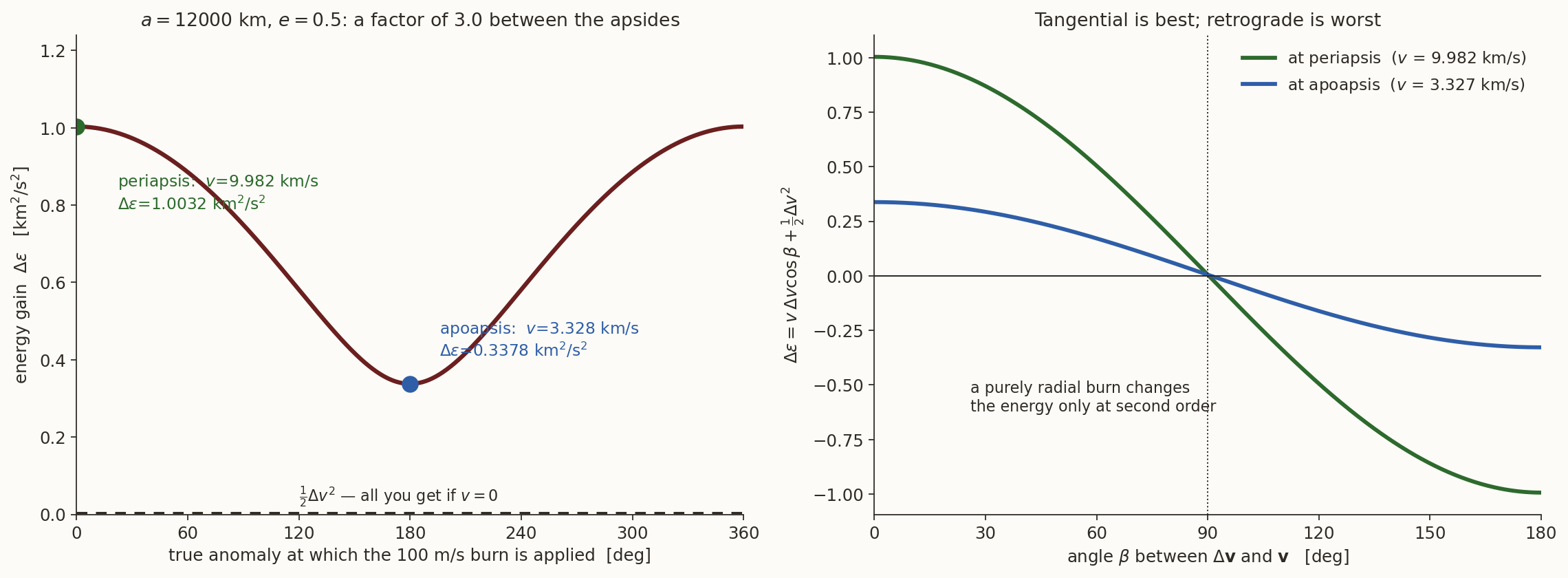
This is why every transfer in the next three parts burns tangentially at an apsis, and why plane changes are made at apoapsis, where \(v\) is small.
3 The Hohmann transfer
3.1 From one circle to another
The most common manoeuvre in practice is a climb (or descent) between two coplanar circular orbits of radii \(r_1<r_2\). The lessons of Section 2.3 tell us what to look for: tangential burns, at points where the transfer orbit’s velocity is parallel to the circles’ velocities. A transfer ellipse that touches both circles has exactly this property: at the touching points the velocities of the circle and of the ellipse are both perpendicular to \(\mathbf r\), so a single tangential impulse switches from one to the other. That ellipse has periapsis \(r_1\) and apoapsis \(r_2\), and the transfer uses half of it (Figure 2).
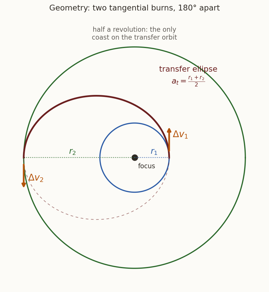
The transfer ellipse has \(a_t=(r_1+r_2)/2\). From vis-viva, \(v^2=\mu(2/r-1/a)\), its speeds at the two ends are
\[ v_{t1}=\sqrt{\mu\left(\frac2{r_1}-\frac1{a_t}\right)}=\sqrt{\frac{2\mu r_2}{r_1(r_1+r_2)}}, \qquad v_{t2}=\sqrt{\frac{2\mu r_1}{r_2(r_1+r_2)}} . \]
Both burns are tangential, so each impulse is just a difference of speeds, with the circular speeds \(v_{c1}=\sqrt{\mu/r_1}\) and \(v_{c2}=\sqrt{\mu/r_2}\):
\[ \boxed{\;\begin{aligned} \Delta v_1&=v_{t1}-v_{c1}=\sqrt{\frac{\mu}{r_1}}\left(\sqrt{\frac{2r_2}{r_1+r_2}}-1\right),\\ \Delta v_2&=v_{c2}-v_{t2}=\sqrt{\frac{\mu}{r_2}}\left(1-\sqrt{\frac{2r_1}{r_1+r_2}}\right). \end{aligned}\;} \tag{3}\]
The transfer takes half the period of the transfer ellipse, \(t_{\rm H}=\pi\sqrt{a_t^3/\mu}\).
History: Hohmann. Walter Hohmann, a German civil engineer, published this transfer in 1925 in Die Erreichbarkeit der Himmelskörper (“The attainability of the heavenly bodies”), decades before any spacecraft flew.
Compute the LEO\(\to\)GEO Hohmann transfer: \(a_t\), \(e_t\), the four speeds, the two impulses, the total and the transfer time. Before you start, guess: is each burn prograde (along the motion) or retrograde?
What you should find
\(a_t=24\,421.07\) km and \(e_t=(r_2-r_1)/(r_2+r_1)=0.72654\).
| speed before | speed after | \(\Delta v\) | |
|---|---|---|---|
| burn 1, at \(r_1\) | \(v_{c1}=7.72576\) | \(v_{t1}=10.15149\) | \(2.42573\) |
| burn 2, at \(r_2\) | \(v_{t2}=1.60784\) | \(v_{c2}=3.07467\) | \(1.46682\) |
Total \(3.89255\) km/s; \(t_{\rm H}=18\,990\) s \(=5.275\) h.
Both burns are prograde. The spacecraft is slower in GEO (\(3.07\) km/s) than in LEO (\(7.73\) km/s), yet every burn adds speed, because it arrives at \(r_2\) moving at only \(1.61\) km/s. Higher orbits are slower but have more energy; the climb itself converts kinetic energy into potential energy.3.2 A farther target can cost less
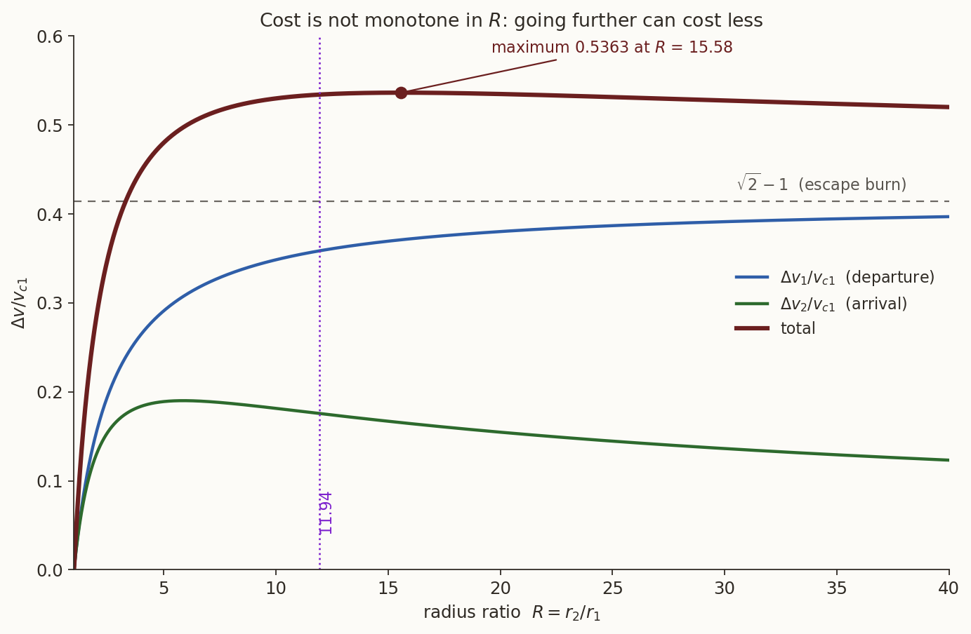
How does the cost grow as the target recedes? Divide Equation 3 by \(v_{c1}\) and write \(R=r_2/r_1\):
\[ \frac{\Delta v_{\rm H}}{v_{c1}}=g(R)= \underbrace{\sqrt{\frac{2R}{1+R}}-1}_{\text{departure}} +\underbrace{\frac1{\sqrt R}\left(1-\sqrt{\frac2{1+R}}\right)}_{\text{arrival}} . \tag{4}\]
Evaluate \(g(R)\) at \(R=6.31\) (LEO to GEO), \(R=15\), \(R=100\) and \(R\to\infty\). What do you notice?
What you should find
\(g(6.31)=0.5038\), \(g(15)=0.5362\), \(g(100)=0.4931\) and \(g(\infty)=\sqrt2-1=0.4142\). The cost rises and then falls: a target \(100\) times farther away is cheaper to reach than one \(15\) times farther away.Why? As \(R\to\infty\) the departure term rises towards \(\sqrt2-1\), which is the escape burn: going very far costs almost exactly as much as leaving for good. Meanwhile the arrival term decays like \(R^{-1/2}\), because the target’s own circular speed decays. Setting \(dg/dR=0\) (numerically) gives the maximum
\[ \boxed{\;\max_R g(R)=0.536258\quad\text{at}\quad R=15.581719 .\;} \tag{5}\]
Beyond \(R=15.58\) the departure burn is already nearly an escape burn and barely grows, while the arrival burn keeps getting cheaper. Keep the number \(15.58\) in mind: it will reappear, unexpectedly, in Section 4.
3.3 Between two ellipses with a common apse line
Real orbits are rarely circular. Suppose both orbits are ellipses in the same plane, sharing a line of apsides. A transfer that is tangential at both ends must still start and end at points where both conics have velocity perpendicular to \(\mathbf r\): the apsides. So the candidates are half-ellipses joining an apsis of orbit 1 to the opposite apsis of orbit 2, and there is always more than one.
3.3.1 Aligned apsides
When the two periapses point the same way (Figure 4), two apsidal transfers exist:
\[ \text{A1}:\ a_t=\frac{r_{p,1}+r_{a,2}}{2},\qquad \text{A2}:\ a_t=\frac{r_{a,1}+r_{p,2}}{2}, \]
that is, A1 joins the periapsis of orbit 1 to the apoapsis of orbit 2, and A2 the apoapsis of 1 to the periapsis of 2.
Each impulse is the difference between the speed of the transfer ellipse and that of the orbit at the burn point, both from vis-viva: \(\Delta v=\left|\sqrt{\mu(2/r-1/a_t)}-\sqrt{\mu(2/r-1/a_{\rm orbit})}\right|\).
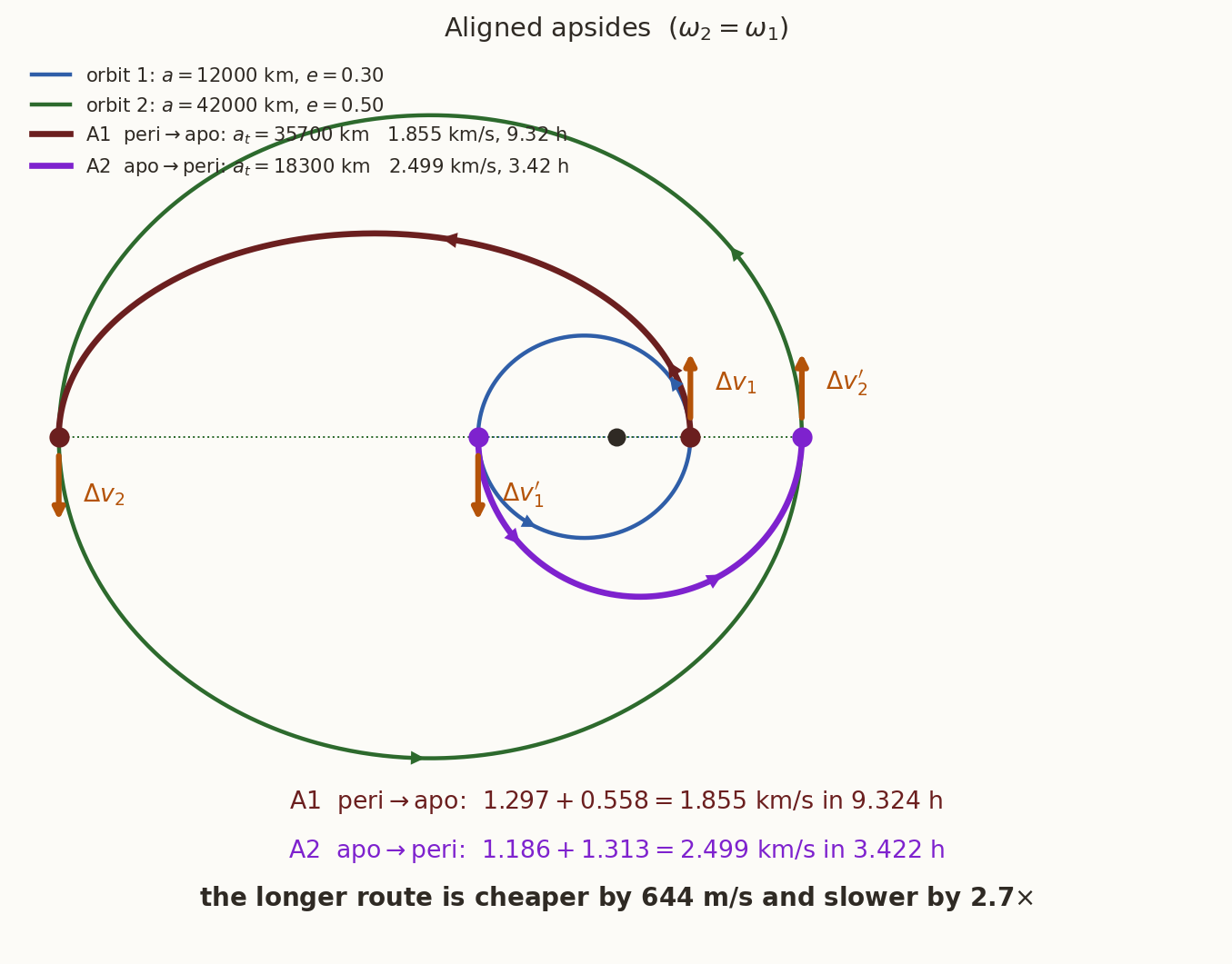
Orbit 1 has \(a_1=12\,000\) km, \(e_1=0.30\); orbit 2 has \(a_2=42\,000\) km, \(e_2=0.50\); apsides aligned. Find the apsidal radii, then the cost and the time of A1 and A2. Before computing, use Section 2.3 to predict which is cheaper.
What you should find
\(r_{p,1}=8400\), \(r_{a,1}=15\,600\), \(r_{p,2}=21\,000\), \(r_{a,2}=63\,000\) km.
| \(a_t\) [km] | \(\Delta v_1\) | \(\Delta v_2\) | total [km/s] | \(t\) [h] | |
|---|---|---|---|---|---|
| A1 \(8400\to63\,000\) | \(35\,700\) | \(1.29675\) | \(0.55850\) | \(\mathbf{1.85525}\) | \(9.324\) |
| A2 \(15\,600\to21\,000\) | \(18\,300\) | \(1.18573\) | \(1.31337\) | \(2.49909\) | \(\mathbf{3.422}\) |
The larger transfer is the cheaper one and the smaller is the quicker one. Reverse the trip and Figure 5 shows the return legs: the same two ellipses, flown the other way.
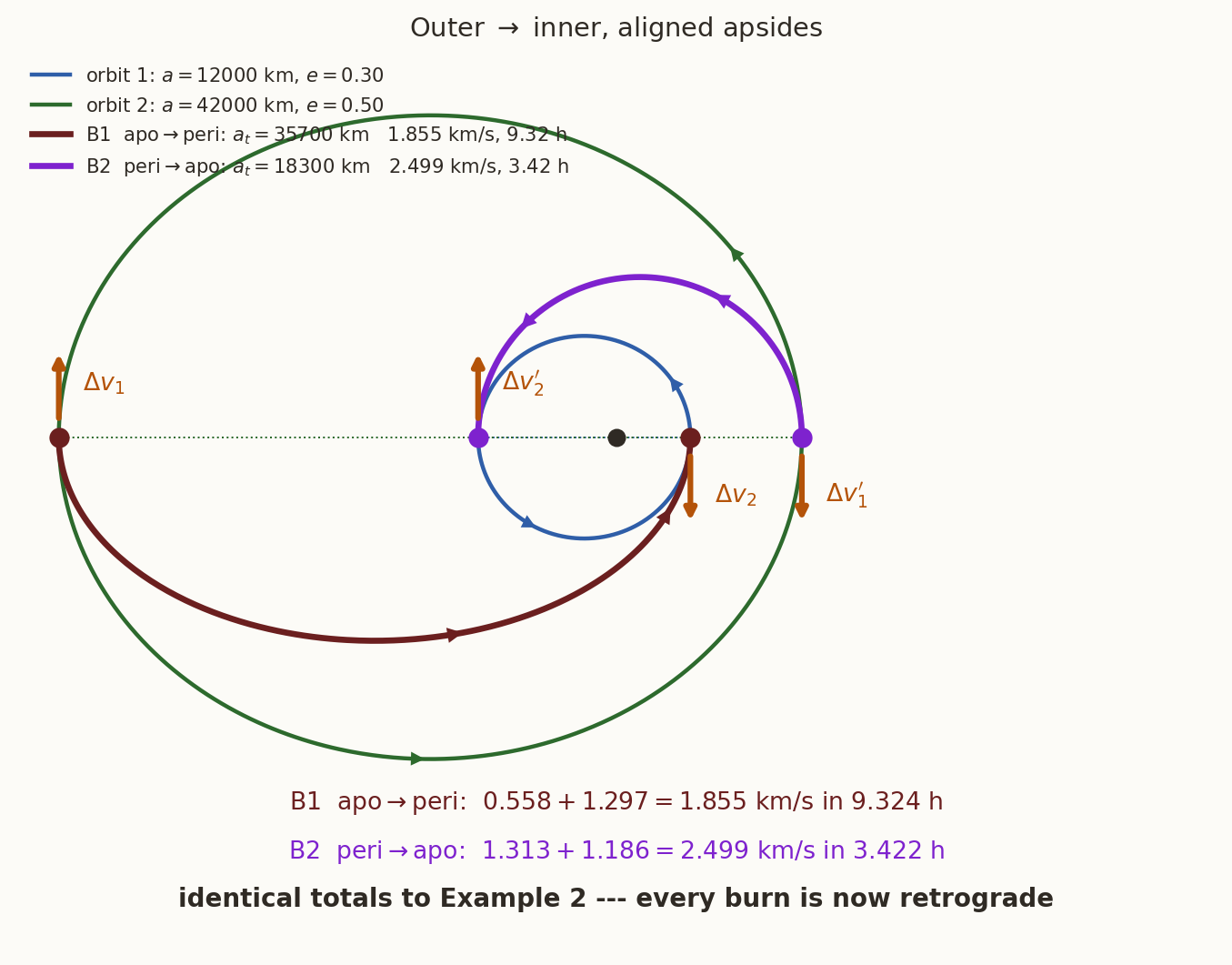
Without computing anything, what do the return legs B1 and B2 cost, and how long do they take?
Answer
Exactly the same as A1 and A2, with the two burns in the opposite order: B1 costs \(0.55850+1.29675=1.85525\) km/s in \(9.324\) h, and B2 costs \(2.49909\) km/s in \(3.422\) h. At each end the two speeds involved, the orbit’s and the transfer’s, do not depend on the direction of travel, and \(|v_{\rm orbit}-v_t|=|v_t-v_{\rm orbit}|\). Only the sense of each impulse flips, from prograde (to climb) to retrograde (to descend). Impulsive \(\Delta v\) is symmetric under time reversal. This is why aerobraking (Section 10) is attractive: the atmosphere can supply a retrograde impulse for free, whereas nothing supplies a prograde one.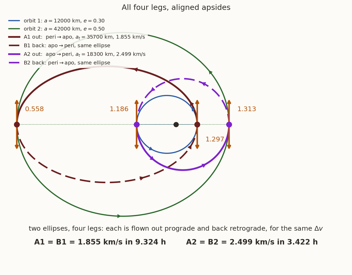
3.3.2 Anti-aligned apsides
Now turn orbit 2 round, \(\omega_2=\omega_1+180^\circ\), so its periapsis is on the opposite side (Figure 7). The apsidal transfers now join the periapses to each other, or the apoapses to each other:
\[ \text{T2}:\ a_t=\frac{r_{p,1}+r_{p,2}}{2},\qquad \text{T1}:\ a_t=\frac{r_{a,1}+r_{a,2}}{2}. \]
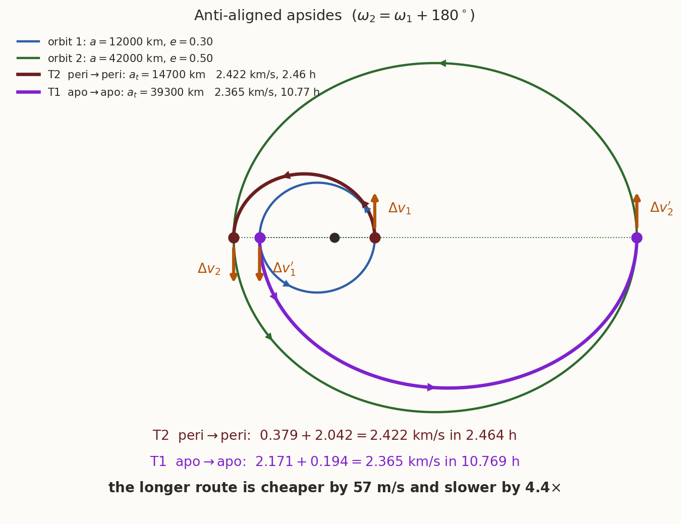
Repeat the previous calculation with the apsides anti-aligned. Which route is cheaper now, and by how much? Compare the cheapest route with the aligned case.
What you should find
| \(a_t\) [km] | \(\Delta v_1\) | \(\Delta v_2\) | total [km/s] | \(t\) [h] | |
|---|---|---|---|---|---|
| T2 \(8400\to21\,000\) | \(14\,700\) | \(0.37924\) | \(2.04250\) | \(2.42174\) | \(\mathbf{2.464}\) |
| T1 \(15\,600\to63\,000\) | \(39\,300\) | \(2.17083\) | \(0.19386\) | \(\mathbf{2.36469}\) | \(10.769\) |
3.3.3 Which route is quicker, and which is cheaper?
Time has a clean answer. Each route is half a revolution of its transfer ellipse, so the one with the larger \(a_t\) is slower. Writing \(c_i=a_ie_i\) for the centre-to-focus distance of orbit \(i\), and using \(r_a-r_p=2ae=2c\),
\[ \underbrace{a_t^{\rm apo\to apo}-a_t^{\rm peri\to peri}=c_1+c_2}_{\text{anti-aligned}}, \qquad \underbrace{a_t^{\rm peri\to apo}-a_t^{\rm apo\to peri}=c_2-c_1}_{\text{aligned}} . \]
With anti-aligned apsides, \(c_1+c_2>0\) always, so the apoapsis-to-apoapsis route is always the slower (here \(c_1+c_2=3600+21\,000=24\,600=39\,300-14\,700\) km). With aligned apsides the slower route is periapsis-to-apoapsis only if the outer orbit is the more offset (\(c_2>c_1\)).
Cost is subtler, because every route sits on the Oberth trade-off: departing deep is efficient, but arriving deep is expensive, since the target orbit is fastest there. Two rules follow: leave the inner orbit at its periapsis, and arrive at the outer orbit at its apoapsis.
- With aligned apsides, A1 obeys both rules, and it is always the cheaper route. A proof follows.
- With anti-aligned apsides the periapsis of orbit 1 and the apoapsis of orbit 2 are on the same side, so no apsidal transfer joins them. T2 obeys the first rule, T1 the second, and which matters more depends on all four radii. Indeed, raising \(e_1\) to \(0.45\) in the example above reverses the order: T2 becomes both cheaper and faster.
Proof that A1 always wins with aligned apsides. (This proof can be skipped on a first reading.) Assume \(r_{p,1}<r_{p,2}\) and \(r_{a,1}<r_{a,2}\). Two facts make the algebra manageable.
- At an apsis \(v=h/r\), so a tangential burn there costs \(|\Delta h|/r\).
- A conic with apsidal radii \(r\) and \(r'\) has \(p=2rr'/(r+r')\), so \(h=\sqrt{\mu p}=\Phi\left(\frac1r+\frac1{r'}\right)\) with \(\Phi(s)=\sqrt{2\mu/s}\).
The radii enter only through their reciprocals, so put \(x_i=1/r_{p,i}\) and \(y_i=1/r_{a,i}\). The hypotheses become \(x_1\ge y_1\), \(x_2\ge y_2\), \(x_1>x_2\) and \(y_1>y_2\). The function \(\Phi\) is decreasing and convex: \(\Phi'<0<\Phi''\). All four burns are prograde, so
\[ \begin{aligned} \Delta v_{A1}&=x_1\left[\Phi(x_1+y_2)-\Phi(x_1+y_1)\right]+y_2\left[\Phi(x_2+y_2)-\Phi(x_1+y_2)\right],\\ \Delta v_{A2}&=y_1\left[\Phi(y_1+x_2)-\Phi(x_1+y_1)\right]+x_2\left[\Phi(x_2+y_2)-\Phi(y_1+x_2)\right]. \end{aligned} \]
Collect the coefficient of each value of \(\Phi\). With \(L(\sigma,\tau)=(\sigma-\tau)\,\Phi(\sigma+\tau)\), which is antisymmetric, \(L(\sigma,\tau)=-L(\tau,\sigma)\),
\[ \Delta v_{A2}-\Delta v_{A1}=L(x_1,y_1)+L(y_1,x_2)+L(x_2,y_2)+L(y_2,x_1), \]
a cyclic sum round \(x_1\to y_1\to x_2\to y_2\to x_1\). Now define the three-term cycle \(C_3(\sigma,\tau,\kappa)=L(\sigma,\tau)+L(\tau,\kappa)+L(\kappa,\sigma)\). It vanishes at \(\sigma=\tau\), and
\[ \frac{\partial C_3}{\partial\sigma}=m(\tau)-m(\kappa),\qquad m(t)=\Phi(\sigma+t)+(\sigma-t)\Phi'(\sigma+t), \]
and \(m'(t)=(\sigma-t)\Phi''(\sigma+t)>0\) for \(t<\sigma\).
So for \(\sigma>\tau>\kappa\), \(C_3>0\) and \(C_3\) increases with its first argument. Adding and subtracting \(L(y_1,y_2)\),
\[ \Delta v_{A2}-\Delta v_{A1}=C_3(x_1,y_1,y_2)+C_3(y_1,x_2,y_2). \]
The first term is positive. If \(r_{a,1}\le r_{p,2}\) then \(y_1\ge x_2>y_2\) and the second is non-negative too. If \(r_{a,1}>r_{p,2}\), reversing the second cycle gives \(\Delta v_{A2}-\Delta v_{A1}=C_3(x_1,y_1,y_2)-C_3(x_2,y_1,y_2)>0\), because \(x_1>x_2\). The two costs are equal only when both orbits are circles, and then both routes are the Hohmann transfer. \(\square\)
For anti-aligned apsides the same bookkeeping gives a sum that is negative when orbit 1 is a circle and positive when orbit 2 is a circle, so it changes sign in between and no general rule exists. Note that the engine of the proof is the convexity of \(\Phi\): the Oberth effect in disguise.
3.4 When the orbits cross
So far one orbit lay inside the other. If instead orbit 1 dips lower at periapsis and reaches higher at apoapsis, the two conics intersect, and a new route opens: a single impulse at a crossing point, with no coast at all. With a shared apse line, a point at true anomaly \(f\) is common to both when
\[ \frac{p_1}{1+e_1\cos f}=\frac{p_2}{1+e_2\cos f} \qquad\Longrightarrow\qquad \boxed{\;\cos f^{*}=\frac{p_2-p_1}{p_1e_2-p_2e_1},\;} \]
with a real crossing when \(|\cos f^{*}|\le1\). The two crossings \(\pm f^{*}\) are mirror images and cost the same.
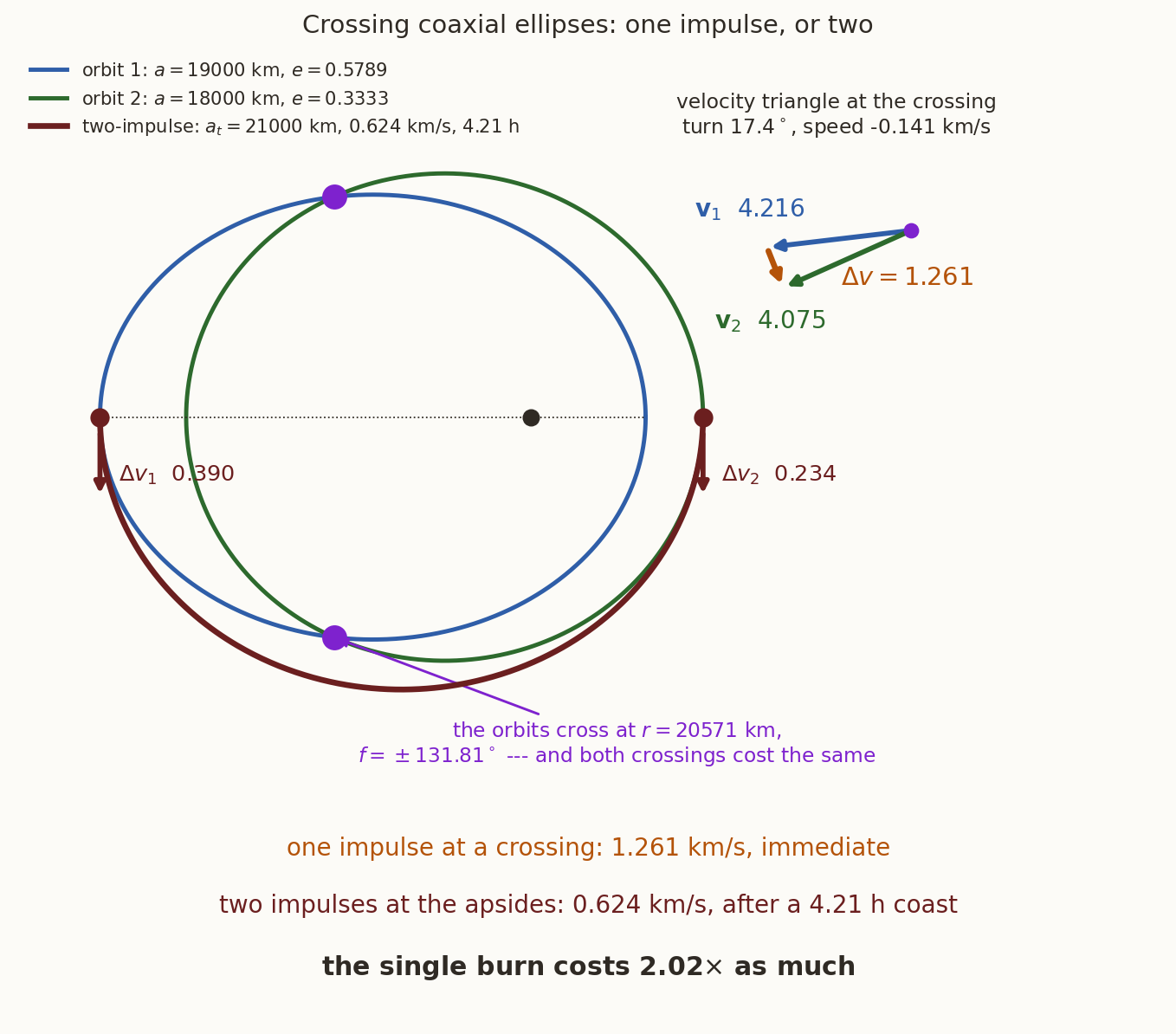
Example. Orbit 1 has \(r_p=8000\), \(r_a=30\,000\) km (\(a_1=19\,000\) km, \(e_1=0.578947\), \(p_1=12\,631.58\) km); orbit 2 has \(r_p=12\,000\), \(r_a=24\,000\) km (\(a_2=18\,000\) km, \(e_2=1/3\), \(p_2=16\,000\) km); apsides aligned. Then
\[ \cos f^{*}=\frac{16\,000-12\,631.58}{12\,631.58\,(0.333333)-16\,000\,(0.578947)}=\frac{3368.42}{-5052.63}=-0.666667, \]
so \(f^{*}=\pm131.81^\circ\) and \(r^{*}=p_1/(1+e_1\cos f^{*})=20\,571.43\) km. With \(v_r=(\mu/h)e\sin f\) and \(v_\theta=h/r\) at that point,
| \(v_r\) | \(v_\theta\) | \(v\) | \(\gamma\) | |
|---|---|---|---|---|
| orbit 1 | \(2.42406\) | \(3.44932\) | \(4.21590\) | \(35.098^\circ\) |
| orbit 2 | \(1.24008\) | \(3.88208\) | \(4.07533\) | \(17.715^\circ\) |
and the single impulse is \(\Delta v=\sqrt{(1.24008-2.42406)^2+(3.88208-3.44932)^2}=1.26058\) km/s.
Now price the two-impulse alternatives: periapsis of 1 (\(8000\) km) to apoapsis of 2 (\(24\,000\) km), and apoapsis of 1 (\(30\,000\) km) to periapsis of 2 (\(12\,000\) km). Which is cheaper, and how does it compare with the single impulse?
What you should find
| \(a_t\) [km] | \(\Delta v_1\) | \(\Delta v_2\) | total [km/s] | \(t\) [h] | |
|---|---|---|---|---|---|
| \(8000\to24\,000\) | \(16\,000\) | \(0.22459\) | \(0.44580\) | \(0.67039\) | \(2.797\) |
| \(30\,000\to12\,000\) | \(21\,000\) | \(0.39018\) | \(0.23358\) | \(\mathbf{0.62376}\) | \(4.206\) |
Why is the single impulse so expensive? At the crossing the two speeds are nearly equal, \(4.216\) against \(4.075\) km/s. Almost the whole \(1.26\) km/s goes into turning the velocity through \(\gamma_1-\gamma_2=17.38^\circ\). A pure turn through \(\theta\) at speed \(\bar v\) costs \(2\bar v\sin(\theta/2)\) (Equation 11); at the mean speed \(\bar v=4.146\) km/s this gives \(1.253\) km/s, \(99\%\) of the exact cost. The single burn is an in-plane version of a plane change. The two-impulse route is cheaper because both of its burns are tangential: they change the size of \(\mathbf v\), not its direction.
3.5 Why Hohmann is optimal
We chose the Hohmann ellipse because it makes both burns tangential. Is there a cheaper two-impulse transfer, with non-tangential burns? The answer is no, and the proof explains why the tangent ellipse wins.
The plan has three steps.
- Write both impulse magnitudes exactly in terms of the transfer orbit’s energy \(\varepsilon\) and angular momentum \(h\) alone.
- In those variables the cost increases with \(\varepsilon\) and decreases with \(h\).
- The transfer conic must reach both radii; this confines \((\varepsilon,h)\) to a region whose boundary has one corner, and the corner is the Hohmann ellipse.
Step 1: the impulses in terms of \((\varepsilon,h)\). At radius \(r_i\) the circular velocity is purely transverse, \((0,\sqrt{\mu/r_i})\) in (radial, transverse) components. The transfer conic has some radial speed \(v_r\) and transverse speed \(v_t=h/r_i\) there. The impulse is the difference:
\[ \Delta v_i^2=v_r^2+\left(v_t-\sqrt{\frac{\mu}{r_i}}\right)^2 =\underbrace{v_r^2+v_t^2}_{v^2}-2v_t\sqrt{\frac{\mu}{r_i}}+\frac{\mu}{r_i}. \]
The radial speed disappears into \(v^2\), which energy already knows: \(v^2=2(\varepsilon+\mu/r_i)\). With \(v_t\sqrt{\mu/r_i}=h\sqrt\mu/r_i^{3/2}\),
\[ \boxed{\;\Delta v_i^2=2\varepsilon+\frac{3\mu}{r_i}-\frac{2h\sqrt\mu}{r_i^{3/2}},\qquad i=1,2.\;} \tag{6}\]
This is exact: no tangency has been assumed. (For a tangential burn, \(v_r=0\) and it reduces to the familiar \(|v-\sqrt{\mu/r_i}|\).)
Step 2: monotonicity. Both \(\Delta v_1^2\) and \(\Delta v_2^2\) increase with \(\varepsilon\) (coefficient \(+2\)) and decrease with \(h\) (coefficient \(-2\sqrt\mu/r_i^{3/2}\)). So the total cost falls as \(h\) grows and as \(\varepsilon\) shrinks.
Step 3: feasibility. The transfer conic must actually reach both radii, which needs a real radial speed there: \(v_r^2=2(\varepsilon+\mu/r)-h^2/r^2\ge0\), i.e.
\[ \varepsilon\ge F(r_i)\equiv\frac{h^2}{2r_i^2}-\frac{\mu}{r_i},\qquad i=1,2 . \]
Since the cost increases with \(\varepsilon\), the optimum has \(\varepsilon=\max\{F(r_1),F(r_2)\}\). Comparing the two bounds,
\[ F(r_2)-F(r_1)=\left(\frac1{r_2}-\frac1{r_1}\right)\left[\frac{h^2}{2}\left(\frac1{r_1}+\frac1{r_2}\right)-\mu\right], \]
and the first bracket is negative, so \(F(r_2)>F(r_1)\) exactly when \(h^2<h_{\rm H}^2\equiv2\mu r_1r_2/(r_1+r_2)\), which is the angular momentum of the Hohmann ellipse. The feasible boundary is two parabolic arcs meeting at \(h=h_{\rm H}\): one corner.
- Case \(h\le h_{\rm H}\): \(\varepsilon=F(r_2)\), so \(v_r=0\) at \(r_2\) (the second burn is tangential) and \(\Delta v_2=\sqrt{\mu/r_2}-h/r_2\), which decreases with \(h\). For the first burn, \(d\Delta v_1/dh=\left(h/r_2^2-\sqrt\mu/r_1^{3/2}\right)/\Delta v_1\), and since \(h\le h_{\rm H}\),
\[ \frac{h}{r_2^2}\le\frac{\sqrt\mu}{r_2^{3/2}}\sqrt{\frac{2r_1}{r_1+r_2}}<\frac{\sqrt\mu}{r_2^{3/2}}<\frac{\sqrt\mu}{r_1^{3/2}}, \]
so it decreases too. The total is smallest at the largest admissible \(h\), \(h=h_{\rm H}\). - Case \(h>h_{\rm H}\): \(\varepsilon=F(r_1)\), the first burn is tangential, \(\Delta v_1=h/r_1-\sqrt{\mu/r_1}\) increases with \(h\), and a similar inequality shows that \(\Delta v_2\) increases too. The total is smallest at the smallest admissible \(h\), again \(h=h_{\rm H}\).
Both cases drive \(h\to h_{\rm H}\), where the conic has periapsis \(r_1\), apoapsis \(r_2\) and two tangential burns: the Hohmann ellipse, the unique minimiser. \(\blacksquare\)
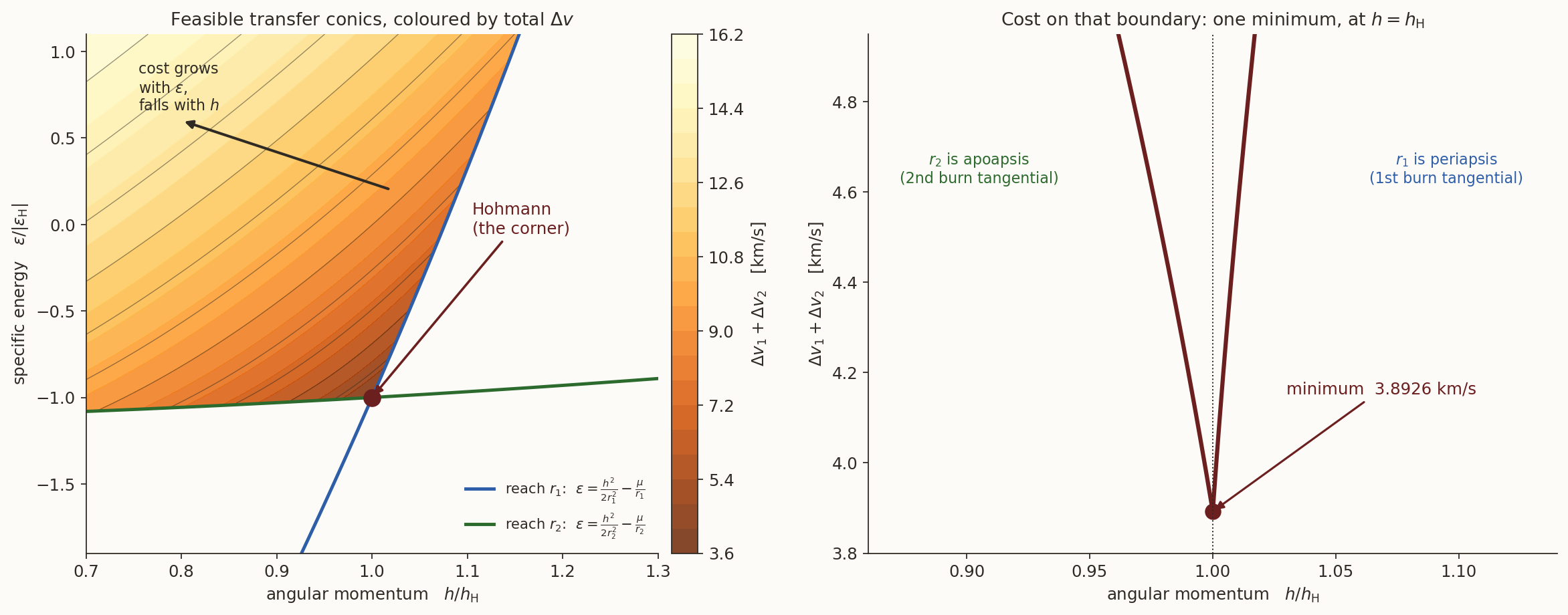
The proof did not assume tangential burns. Where did tangency come from?
Answer
From the feasibility constraint becoming active. The cost wants large \(h\) and small \(\varepsilon\); the requirement to reach a radius forbids \(\varepsilon\) from being too small for a given \(h\). On the active constraint \(v_r=0\) at that radius, i.e. the burn there is tangential. At the corner both constraints are active, so both burns are tangential.4 The bi-elliptic transfer
4.1 Three burns can beat two
The optimality theorem is about two impulses. Can three do better? Figure 3 suggests how: for large \(R\), the departure burn is nearly an escape burn anyway, so overshooting the target is almost free; and far from the Earth the spacecraft is slow, so changes made there are cheap. The bi-elliptic transfer exploits both: burn 1 raises apoapsis to a distant \(r_b>r_2\); burn 2, at \(r_b\), raises periapsis from \(r_1\) to \(r_2\); burn 3, at \(r_2\), circularises (Figure 10).
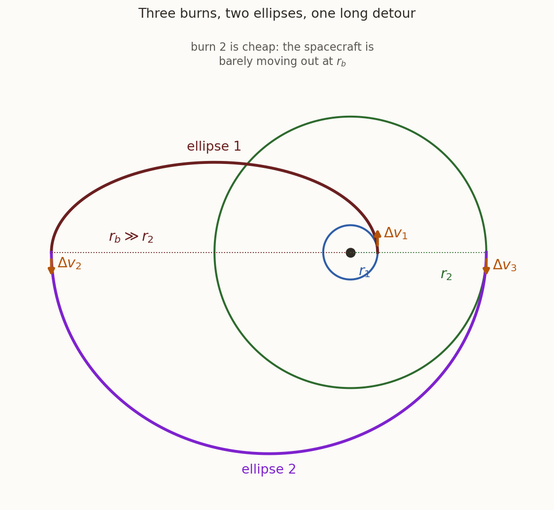
With \(R=r_2/r_1\), \(R^{*}=r_b/r_1\ge R\) and every speed divided by \(v_{c1}\), vis-viva on the two ellipses gives
\[ \frac{\Delta v_1}{v_{c1}}=\sqrt{\frac{2R^{*}}{1+R^{*}}}-1, \qquad \frac{\Delta v_2}{v_{c1}}=\sqrt{\frac2{R^{*}}}\left(\sqrt{\frac{R}{R+R^{*}}}-\sqrt{\frac1{1+R^{*}}}\right), \]
\[ \frac{\Delta v_3}{v_{c1}}=\sqrt{\frac{2R^{*}}{R(R+R^{*})}}-\frac1{\sqrt R}\qquad\text{(retrograde).} \tag{7}\]
The key is \(\Delta v_2\): it carries the factor \(\sqrt{2/R^{*}}\), so as \(r_b\to\infty\) the cost of moving the periapsis by any amount tends to zero. Setting \(R^{*}=R\) makes \(\Delta v_3=0\) and gives back the Hohmann transfer exactly, so the bi-elliptic family is a continuous extension of Hohmann.
Take \(R=15\) (\(r_2=100\,172.06\) km) and \(r_b=400\,000\) km. Compute the three burns, the total, the Hohmann cost and the two transfer times.
What you should find
\(a_{t1}=(r_1+r_b)/2=203\,339\) km and \(a_{t2}=(r_2+r_b)/2=250\,086\) km.
| burn | where | from | to | \(\Delta v\) |
|---|---|---|---|---|
| 1 | \(r_1\) | \(7.72576\) | \(10.83580\) | \(3.11004\) |
| 2 | \(r_b\) | \(0.18091\) | \(0.63178\) | \(0.45088\) |
| 3 | \(r_2\) | \(2.52279\) | \(1.99478\) | \(0.52801\) |
4.2 The two thresholds
When does the bi-elliptic transfer win? Two different questions have two different answers.
- Does the limiting case \(r_b\to\infty\) beat Hohmann? Taking the limit term by term, \(\Delta v_{\rm bi,\infty}/v_{c1}=(\sqrt2-1)(1+1/\sqrt R)\). Equating this to \(g(R)\) and solving numerically gives \(\boxed{R^{\dagger}=11.938765}\).
- Does any \(r_b>r_2\) beat Hohmann? That is, is \(\partial\Delta v_{\rm bi}/\partial R^{*}<0\) at \(R^{*}=R\)? The answer is yes for \(R>R^{\ddagger}=15.581719\).
So: for \(R<11.94\) Hohmann always wins; for \(11.94<R<15.58\) the bi-elliptic wins only if \(r_b\) is large enough; for \(R>15.58\) it wins for every \(r_b>r_2\).
\(15.581719\) is exactly the maximum of the Hohmann cost curve, Equation 5. Coincidence?
Answer
No. Differentiate \(\Delta v_2+\Delta v_3\) of Equation 7 with respect to \(R\) and set \(R^{*}=R\). The first impulse does not involve \(R\), and the other two give
\[ \begin{aligned} \frac{\partial}{\partial R}\left[\sqrt{\frac2{R^{*}}}\sqrt{\frac{R}{R+R^{*}}}\right]_{R^{*}=R}&=\frac1{4R^{3/2}},\\ \frac{\partial}{\partial R}\left[\sqrt{\frac{2R^{*}}{R(R+R^{*})}}-\frac1{\sqrt R}\right]_{R^{*}=R}&=-\frac1{4R^{3/2}}, \end{aligned} \]
which cancel. So \(\partial\Delta v_{\rm bi}/\partial R=0\) at \(R^{*}=R\) for every \(R\). Differentiating the identity \(\Delta v_{\rm bi}(R,R)=\Delta v_{\rm H}(R)\) with the chain rule then gives \(\partial\Delta v_{\rm bi}/\partial R^{*}|_{R^{*}=R}=d\Delta v_{\rm H}/dR\). A detour beyond \(r_2\) pays exactly when the Hohmann cost is decreasing in \(R\), i.e. beyond its maximum. The two numbers quoted in textbooks are the same number twice.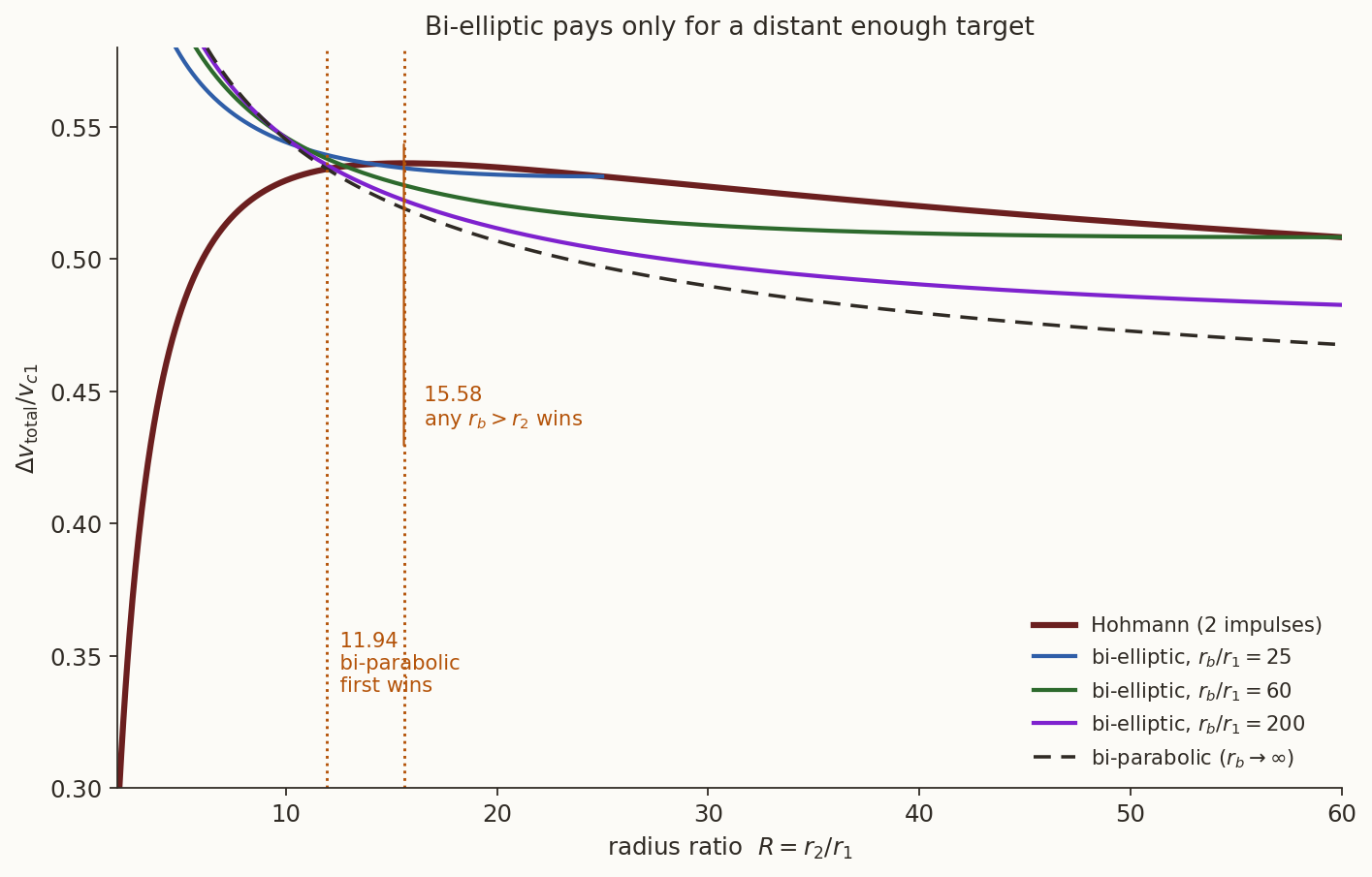
The curves in Figure 11 do not merge. Between \(R=14.10\) and \(R=25\) the \(r_b=25r_1\) curve lies strictly below Hohmann, by at most \(0.0030\,v_{c1}\) (\(0.56\%\)) near \(R=18.5\), and the two meet only at \(R=25\), where \(r_b=r_2\) and the “bi-elliptic” is the Hohmann transfer.
LEO to GEO has \(R=6.31\). Is the bi-elliptic transfer useful for putting satellites in GEO?
Answer
No: \(R=6.31\) is well below \(11.94\), so Hohmann wins whatever \(r_b\). The bi-elliptic transfer pays only for large \(R\), and even then the saving is a percent or two, against a time penalty of days or weeks.4.3 A stopover is not a bi-elliptic
What if the intermediate burn is made short of the target, \(r_b<r_2\)? It is still a three-impulse manoeuvre, but the geometry changes in one decisive way. Ellipse 2 now runs from its periapsis \(r_b\) out to its apoapsis \(r_2\), so burn 2 must raise the apoapsis (an energy change, at low speed), and the spacecraft arrives at \(r_2\) below circular speed, so burn 3 is prograde:
\[ \frac{\Delta v_3}{v_{c1}}=\frac1{\sqrt R}-\sqrt{\frac{2R^{*}}{R(R+R^{*})}}>0\qquad(R^{*}<R). \]
(So the bi-elliptic formula Equation 7 does not apply here: summed blindly it would subtract the third burn instead of adding it.)
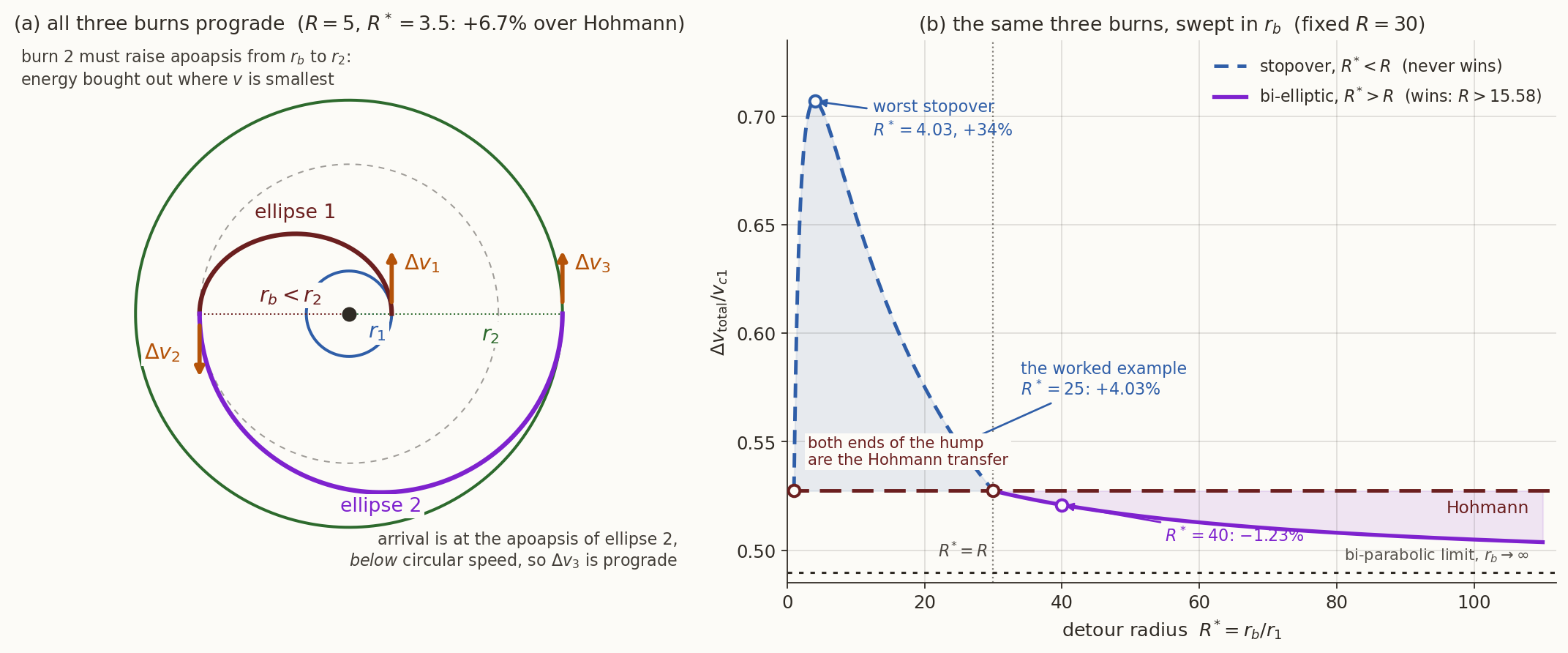
At both ends of the range the stopover is the Hohmann transfer (\(R^{*}=1\) puts the first burn at \(r_1\) and \(R^{*}=R\) circularises on arrival), and everything in between is worse: for \(R=30\) the worst choice is \(R^{*}=4.02\), costing \(34\%\) more. The reason is Equation 2 again. Burn 2 must now supply energy, and \(r_b\) is a poor place to do it, because \(v\) is small there. The bi-elliptic transfer is cheap because its far burn changes the periapsis, which costs almost nothing.
Price a stopover with \(R=30\) and \(r_b=25r_1\). Burn 1 turns out cheaper than Hohmann’s first burn. Where does the extra cost come from?
What you should find
\(r_2=200\,344.11\) km, \(r_b=166\,953.43\) km, \(a_{t1}=86\,815.78\) km, \(a_{t2}=183\,648.77\) km.
| burn | where | from | to | \(\Delta v\) |
|---|---|---|---|---|
| 1 | \(r_1\) | \(7.72576\) | \(10.71370\) | \(2.98794\) |
| 2 | \(r_b\) | \(0.42855\) | \(1.61386\) | \(1.18531\) |
| 3 | \(r_2\) | \(1.34488\) | \(1.41052\) | \(0.06564\) |
Total \(4.23889\) km/s against Hohmann’s \(4.07470\) km/s: \(+4.03\%\), and \(6.01\) days instead of \(1.92\).
Burn 1 saves \(34.5\) m/s (\(2.98794\) against \(3.02245\)) by not climbing the last \(33\,391\) km. Burns 2 and 3 together then cost \(198.7\) m/s more than Hohmann’s single arrival burn, because the missing energy is bought at \(r_b\), where the spacecraft moves at \(429\) m/s instead of the \(10.71\) km/s it had at \(r_1\). By conservation of angular momentum the ratio of those two speeds is exactly \(r_b/r_1=25\), so each m/s buys \(25\) times less energy there. (The same three-burn structure with \(r_b=40r_1\), a genuine bi-elliptic, costs \(4.02458\) km/s, \(1.2\%\) less than Hohmann.)5 Phasing
5.1 Catching up on the same orbit
A chaser and its target are on the same circular orbit, but the chaser trails by an angle \(\Delta\theta\). How does it catch up? The instinct, “speed up”, is wrong: a prograde burn raises the orbit, a higher orbit has a longer period, and the chaser falls further behind. The right move is counter-intuitive: burn retrograde, drop onto a smaller ellipse with a shorter period, go round once (or several times), and arrive back at the burn point early, exactly when the target arrives there. A second, equal and opposite burn restores the circular orbit (Figure 13).
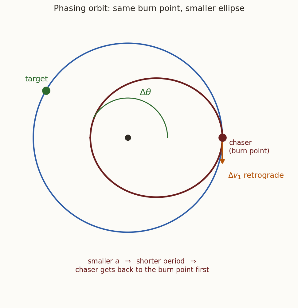
To close the gap in \(k\) revolutions, the chaser must complete \(k\) phasing orbits in the time the target takes to cover \(2\pi k-\Delta\theta\):
\[ kT_{ph}=kT-\frac{\Delta\theta}{2\pi}T \qquad\Longrightarrow\qquad \boxed{\;T_{ph}=T\left(1-\frac{\Delta\theta}{2\pi k}\right),\;} \]
where \(T\) is the period of the circular orbit of radius \(r\). Kepler’s third law converts the period into a semi-major axis, \(a_{ph}=r\,(T_{ph}/T)^{2/3}\). The burn point is the apoapsis of the phasing ellipse, so
\[ \boxed{\;\Delta v_{\rm total}=2\left|\sqrt{\mu\left(\frac2r-\frac1{a_{ph}}\right)}-\sqrt{\frac{\mu}{r}}\right|.\;} \tag{8}\]
A chaser at \(r=6778\) km (the space station’s altitude) is \(10^\circ\) behind its target. Close the gap in one revolution (\(k=1\)). Find \(T\), \(T_{ph}\), \(a_{ph}\), the perigee altitude of the phasing ellipse and the total \(\Delta v\).
What you should find
\(T=5553.46\) s \(=92.558\) min, \(T_{ph}=T(1-1/36)=5399.19\) s, \(a_{ph}=6778(35/36)^{2/3}=6651.89\) km, so the perigee is at \(2a_{ph}-r=6525.79\) km, i.e. \(147.6\) km altitude. The speeds are \(v_c=7.668636\) and \(v_{ph}=7.595597\) km/s, so \(\Delta v_{\rm total}=2(0.073039)=146.1\) m/s.A perigee at \(147.6\) km is inside the atmosphere: the chaser would re-enter. What is the remedy, and what does it cost?
Answer
Use more phasing revolutions. With \(k=3\), \(a_{ph}=6736.10\) km, the perigee altitude is \(316\) km, and \(\Delta v_{\rm total}=47.8\) m/s: one third of the cost, with a safe perigee. The cost falls roughly as \(1/k\), because the period change per orbit is \(k\) times smaller. In phasing, time is the cheapest resource, which is why rendezvous profiles take hours or days.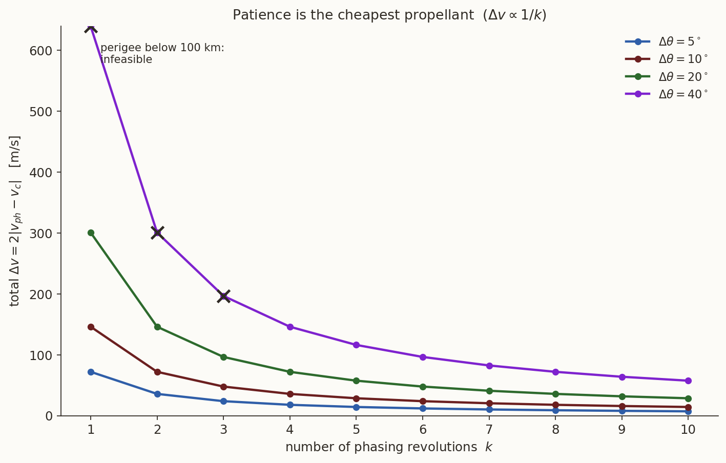
5.2 Phasing on an ellipse: where to burn?
A spacecraft on an ellipse \((a,e)\) must arrive somewhere \(\Delta t\) later than it otherwise would. One extra-long orbit does it, with \(T_{ph}=T+\Delta t\) and \(a_{ph}=a(1+\Delta t/T)^{2/3}\). But now the burn point matters: an ellipse has a fast end and a slow end. Differentiate vis-viva at fixed \(r\):
\[ v^2=\mu\left(\frac2r-\frac1a\right) \quad\Longrightarrow\quad 2v\,dv=\frac{\mu}{a^2}\,da \quad\Longrightarrow\quad \boxed{\;dv=\frac{\mu}{2va^2}\,da .\;} \tag{9}\]
For a prescribed \(da\), the impulse is inversely proportional to the speed at the burn point: phase at periapsis. The ratio of costs between the two apsides is \(v_p/v_a=(1+e)/(1-e)\).
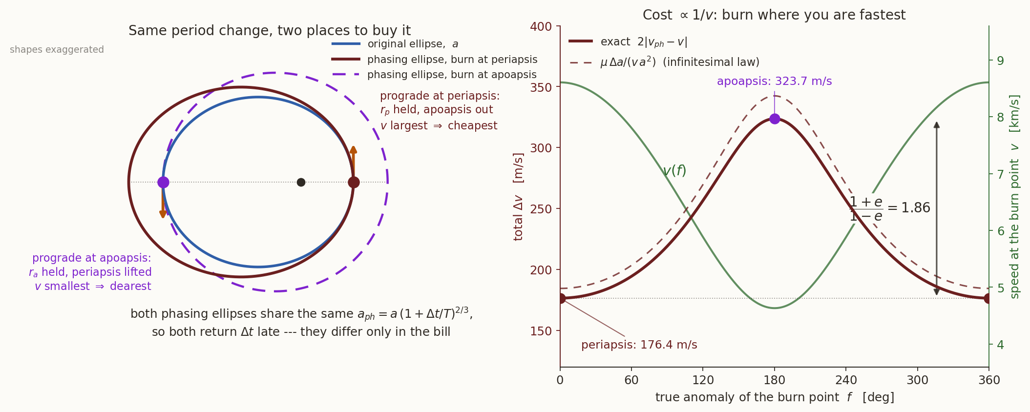
A spacecraft on an orbit with \(a=10\,000\) km and \(e=0.3\) must arrive \(600\) s late. Compare the cost of doing it at periapsis and at apoapsis (two equal burns each time).
What you should find
\(T=9952.01\) s and \(a_{ph}=10\,000(1+600/9952.01)^{2/3}=10\,397.99\) km.
| burn at | \(v\) before | \(v\) after | \(\Delta v\) (each) | total |
|---|---|---|---|---|
| periapsis, \(r=7000\) | \(8.603825\) | \(8.692036\) | \(0.088211\) | \(\mathbf{0.17642}\) |
| apoapsis, \(r=13\,000\) | \(4.632829\) | \(4.794662\) | \(0.161834\) | \(0.32367\) |
6 Rotating the apse line
6.1 A purely radial impulse
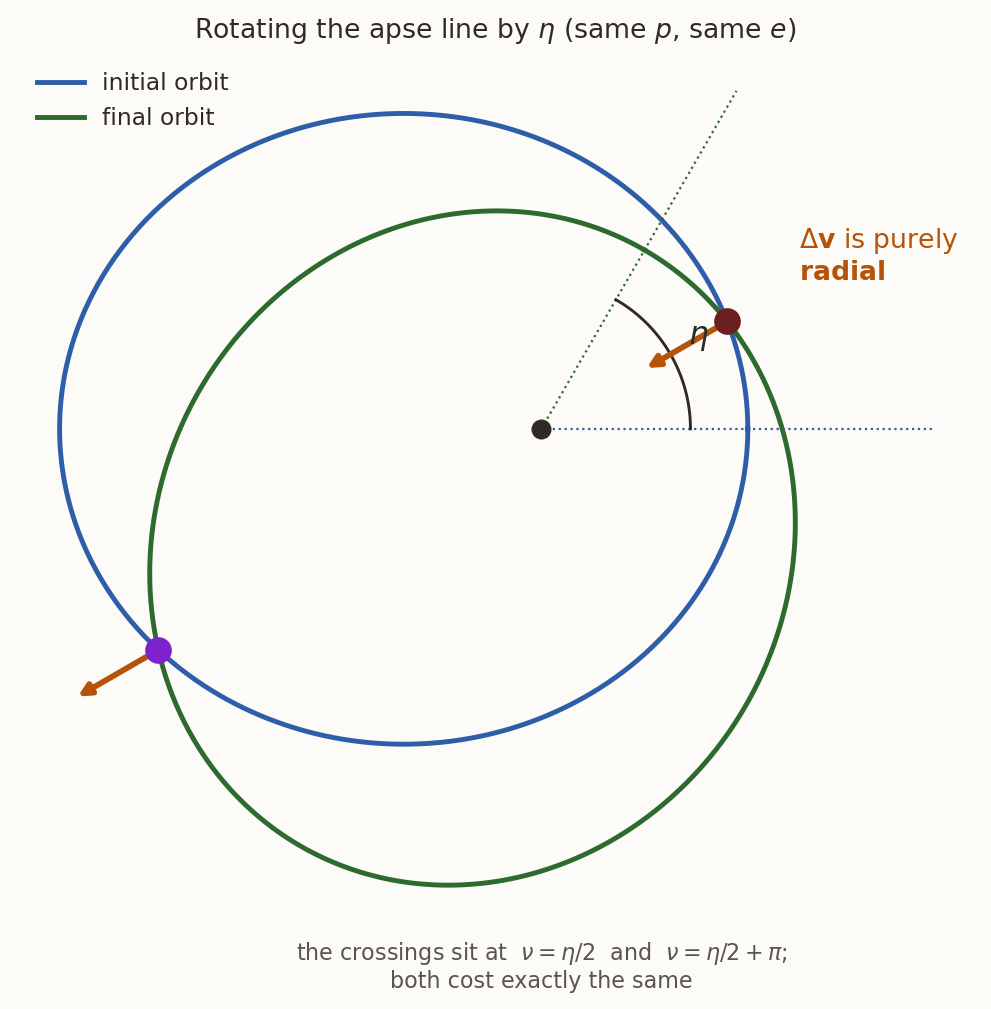
Suppose we want to turn the orbit’s line of apsides by an angle \(\eta\), keeping its size and shape: same \(p\) and \(e\), new argument of periapsis \(\omega+\eta\). The two orbits cross (they have the same size, so they must), and at a crossing a single impulse can switch from one to the other (Figure 16).
A point at true anomaly \(f\) on the first orbit is at \(f-\eta\) on the second. Equal radii require
\[ \frac{p}{1+e\cos f}=\frac{p}{1+e\cos(f-\eta)} \quad\Longrightarrow\quad \cos f=\cos(f-\eta), \]
whose solutions (other than the trivial \(\eta=0\)) are \(f=\eta/2\) and \(f=\eta/2+\pi\).
At the first crossing the initial orbit has \(f=\eta/2\) and the final orbit has \(f'=-\eta/2\). With \(v_r=\sqrt{\mu/p}\,e\sin f\) and \(v_\theta=\sqrt{\mu/p}\,(1+e\cos f)\),
Use the parity of cosine and sine to compare \((v_r,v_\theta)\) on the two orbits at the crossing. What is the impulse?
What you should find
\(\cos\) is even and \(\sin\) is odd, so \(v_\theta'=v_\theta\) and \(v_r'=-v_r\). The transverse components agree and the radial ones are opposite, so \(\Delta\mathbf v=-2v_r\,\hat{\mathbf r}\): purely radial.\[ \boxed{\;\Delta v=2\sqrt{\frac{\mu}{p}}\,e\sin\frac\eta2=2v\sin\gamma ,\;} \tag{10}\]
where \(\gamma\) is the flight path angle at the crossing. The second form is worth seeing geometrically: the impulse leaves the speed unchanged and reflects \(\mathbf v\) in the local horizontal (\(\gamma\to-\gamma\)). It turns \(\mathbf v\) through \(2\gamma\) at constant speed, the same isosceles triangle as a plane change (Equation 11), so \(\Delta v=2v\sin(2\gamma/2)\).
Equation 10 contains no \(r\). The two crossings are at very different radii; which is cheaper?
Answer
Neither: both cost the same. At the second crossing \(v\) is smaller but \(|\gamma|\) larger, and the product \(v|\sin\gamma|=|v_r|\) is the same. For the example below: \(v=8.742\) km/s, \(\gamma=4.271^\circ\) at \(f=15^\circ\), and \(v=3.913\) km/s, \(\gamma=-9.576^\circ\) at \(f=195^\circ\); both give \(1.30204\) km/s.Example. \(a=12\,000\) km, \(e=0.4\), so \(p=10\,080\) km and \(\sqrt{\mu/p}=6.288378\) km/s; rotate by \(\eta=30^\circ\). At \(f=15^\circ\), \(r=7270.79\) km, \(v_r=0.651021\), \(v_\theta=8.718020\), and
\[ \Delta v=2(0.651021)=1.30204\ \text{km/s},\qquad\gamma=\arctan\frac{v_r}{v_\theta}=4.271^\circ . \]
6.2 Going round instead
There is a two-burn alternative: circularise at apoapsis, then, at the right point of the circle, re-eccentricise with the apse line in the new direction. Its cost does not depend on \(\eta\) at all.
For the same orbit, compute the cost of the two-burn route, and the rotation angle \(\eta\) above which it beats the single radial impulse.
What you should find
At \(r_a=16\,800\) km, \(v_c=4.870956\) and \(v_a=3.773027\) km/s, so \(\Delta v_{\rm alt}=2(4.870956-3.773027)=2.19586\) km/s. Setting \(2\sqrt{\mu/p}\,e\sin(\eta/2)=2.19586\) gives \(\eta_{\rm cross}=51.8^\circ\). Below it (\(30^\circ\): \(1.30\) km/s) rotate directly; above it (\(180^\circ\) would cost \(5.03\) km/s) go via the circle.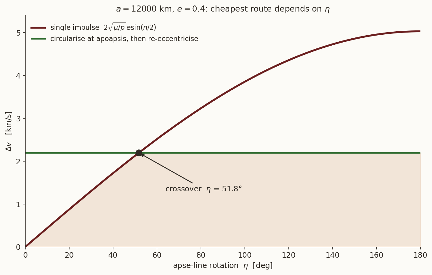
A direct rotation costs \(\propto\sin(\eta/2)\) and grows without saturating at a small value, while the detour costs a constant. Large reorientations are made by changing the shape of the orbit, not by rotating it.
7 Rendezvous
Phasing (Section 5) brings a chaser to the right place on the right orbit at the right time when the two spacecraft share an orbit. In general they do not, and two further tools are needed, each with its own note.
- Far away, with separations comparable to the orbit, the question is “which conic joins these two positions in this time?”. That is Lambert’s problem: see the Lambert note. A Lambert arc between two circles that is forced to be faster than Hohmann costs more, and the cheapest Lambert arc over all transfer times is never cheaper than Hohmann, as the optimality theorem requires.
- Close in, within a few kilometres of the target, the motion is best described in a frame that rotates with the target, where it obeys the linear Clohessy–Wiltshire equations: see the CW note. There the counter-intuitive rule of Section 5 appears in its purest form: to move forward along the track, burn radially inward or backward, not forward.
8 Plane changes
8.1 The cost of turning the plane
To change the orbital plane, the velocity must be rotated out of the old plane into the new one. The burn must happen on the line of nodes, the line where the two planes intersect, because only there is the spacecraft on both orbits at once. If the speed is to stay the same, the velocity triangle is isosceles, with legs \(v\) and apex angle \(\Delta i\) (Figure 18):
\[ \Delta v^2=v^2+v^2-2v^2\cos\Delta i=4v^2\sin^2\frac{\Delta i}2 , \]
so
\[ \boxed{\;\Delta v=2v\sin\frac{\Delta i}2 .\;} \tag{11}\]
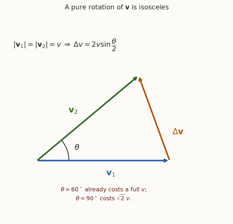
What does a \(60^\circ\) plane change cost? A \(180^\circ\) one?
Answer
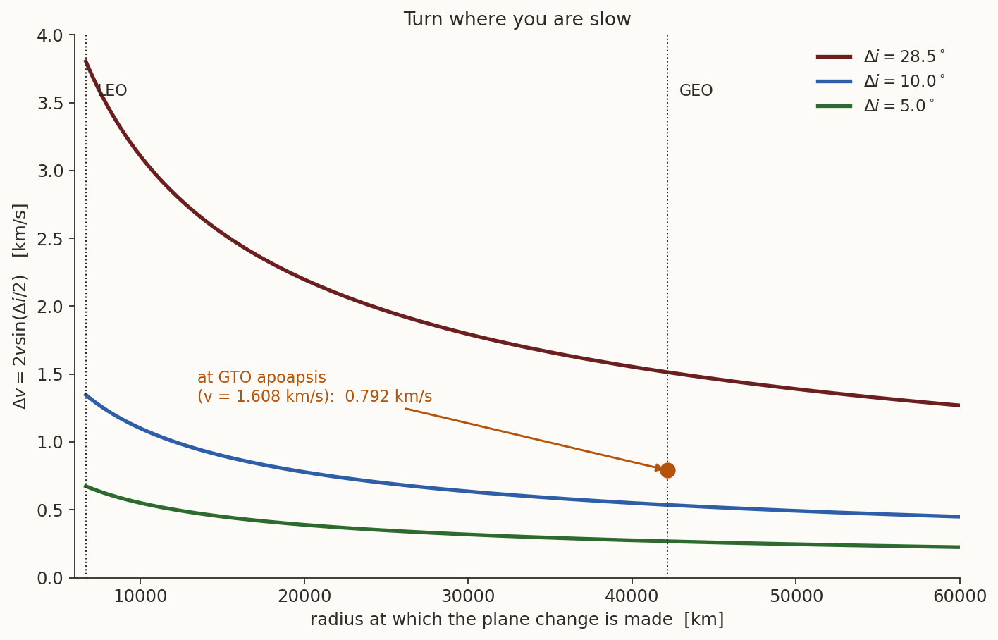
\(2v\sin30^\circ=v\): a full orbital speed. \(2v\sin90^\circ=2v\): reversing the orbit means stopping and starting again. Large plane changes are never cheap.The cost is proportional to \(v\), the opposite of the Oberth effect: change planes where the speed is small.
A launch from Cape Canaveral leaves a satellite in an orbit inclined \(28.5^\circ\); it is wanted in the equatorial plane. Compute the cost of the \(28.5^\circ\) plane change (a) in LEO, (b) in GEO, (c) at the apoapsis of the LEO\(\to\)GEO transfer ellipse.
What you should find
| where | \(v\) [km/s] | \(\Delta v\) [km/s] |
|---|---|---|
| LEO, \(r=6678\) km | \(7.72576\) | \(3.80344\) |
| GEO, \(r=42\,164\) km | \(3.07467\) | \(1.51368\) |
| apoapsis of the transfer ellipse | \(1.60784\) | \(\mathbf{0.79155}\) |
8.2 Combining the plane change with a transfer burn
A transfer burn must be made anyway. If the plane change is made in the same burn, the cost is the magnitude of a sum instead of a sum of magnitudes. With the angle between the arriving velocity \(\mathbf v_{t2}\) and the final velocity \(\mathbf v_{c2}\) equal to \(\Delta i\), the law of cosines gives
\[ \boxed{\;\Delta v_2=\sqrt{v_{t2}^2+v_{c2}^2-2v_{t2}v_{c2}\cos\Delta i}\;} \]
For LEO\(\to\)GEO with \(\Delta i=28.5^\circ\), compare three strategies: (a) Hohmann, then a separate plane change in GEO; (b) the whole plane change folded into the LEO burn; (c) the whole plane change folded into the GEO burn.
What you should find
| strategy | \(\Delta v\) [km/s] |
|---|---|
| (a) Hohmann, then a separate plane change in GEO | \(3.89255+1.51368=5.40623\) |
| (b) plane change folded into the LEO burn | \(4.98923+1.46682=6.45606\) |
| (c) plane change folded into the GEO burn | \(2.42573+1.83023=\mathbf{4.25596}\) |
8.3 Sharing the turn between two burns
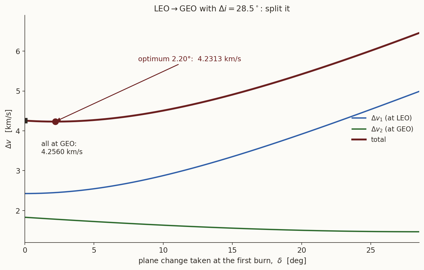
Should all of the turn go into the second burn? Give an angle \(\delta\) to the first burn and \(\Delta i-\delta\) to the second:
\[ \Delta v(\delta)= \underbrace{\sqrt{v_{c1}^2+v_{t1}^2-2v_{c1}v_{t1}\cos\delta}}_{\Delta v_1,\ \text{at }r_1} +\underbrace{\sqrt{v_{t2}^2+v_{c2}^2-2v_{t2}v_{c2}\cos(\Delta i-\delta)}}_{\Delta v_2,\ \text{at }r_2} . \]
Differentiating each square root,
\[ \frac{d\Delta v}{d\delta}=\frac{v_{c1}v_{t1}\sin\delta}{\Delta v_1}-\frac{v_{t2}v_{c2}\sin(\Delta i-\delta)}{\Delta v_2}, \]
and the optimum satisfies
\[ \boxed{\;\frac{v_{c1}v_{t1}\sin\delta}{\Delta v_1}=\frac{v_{t2}v_{c2}\sin(\Delta i-\delta)}{\Delta v_2}.\;} \]
Evaluate \(d\Delta v/d\delta\) at \(\delta=0\). What does its sign tell you?
Answer
At \(\delta=0\) the first term vanishes and the second is negative, so \(d\Delta v/d\delta<0\): moving a little of the turn into the first burn always reduces the cost. The reason is that for small \(\delta\) the first burn’s cost grows only quadratically (\(\Delta v_1\) is mainly the tangential speed change, and a small tilt adds to it at second order), while the second burn’s saving is first order.Solving numerically for LEO\(\to\)GEO with \(\Delta i=28.5^\circ\): \(\delta^{*}=2.20^\circ\), \(\Delta v_1=2.44945\), \(\Delta v_2=1.78186\), total \(4.23131\) km/s (both sides of the optimality condition equal \(1.22925\)). That is a further \(24.7\) m/s below strategy (c), for nothing, and it is standard practice on missions to geostationary orbit.
8.4 Changing the node instead
A change of the right ascension of the ascending node, \(\Delta\Omega\), at fixed inclination \(i\) also turns the orbital plane. By how much? The unit normal of an orbit with inclination \(i\) and node \(\Omega\) is \(\hat{\mathbf h}=(\sin i\sin\Omega,\ -\sin i\cos\Omega,\ \cos i)\) (see the orbital-elements note). The angle \(\alpha\) between the two planes is the angle between their normals:
\[ \cos\alpha=\hat{\mathbf h}_1\cdot\hat{\mathbf h}_2=\sin^2i\left(\sin\Omega_1\sin\Omega_2+\cos\Omega_1\cos\Omega_2\right)+\cos^2i, \]
\[ \boxed{\;\cos\alpha=\cos^2i+\sin^2i\cos\Delta\Omega,\qquad\Delta v=2v\sin\frac\alpha2 .\;} \]
(The burn is made where the two planes intersect. On a circular orbit the velocity there is perpendicular to that line and turns through the full \(\alpha\); on an eccentric orbit the radial part of \(\mathbf v\) lies along the line and is untouched, so the formula over-estimates.)
Check the formula for a polar orbit (\(i=90^\circ\)) and an equatorial one (\(i\to0\)).
Answer
For \(i=90^\circ\), \(\cos\alpha=\cos\Delta\Omega\), so \(\alpha=\Delta\Omega\): polar orbit planes all meet at the poles, and changing the node is the whole turn. For \(i\to0\), \(\alpha\to0\): an equatorial orbit has no node to move.The space station orbits at \(r=6778\) km with \(i=51.6^\circ\). What does a \(10^\circ\) node change cost? Then compare with simply waiting: the Earth’s oblateness makes the node drift at \(\dot\Omega=-\frac32J_2\left(R_\oplus/p\right)^2n\cos i\), with \(J_2=1.0826\times10^{-3}\) and \(n\) the mean motion.
What you should find
\(\cos\alpha=\cos^2 51.6^\circ+\sin^2 51.6^\circ\cos10^\circ=0.990669\), so \(\alpha=7.833^\circ\) and \(\Delta v=2(7.668636)\sin3.9165^\circ=1.0476\) km/s.
The drift is \(\dot\Omega=-5.0027^\circ\)/day, so \(10^\circ\) of node takes \(2.0\) days, for nothing. A launch that misses its node waits; it does not burn. (A spacecraft that wants the node to move the other way can still exploit \(J_2\), by parking for a while on an orbit of different altitude or inclination where the drift rate differs.)9 Escape
9.1 Where to burn
A spacecraft on an elliptic orbit wants to leave the planet. Where should it burn? Escape means reaching zero energy, i.e. raising the speed at radius \(r\) to \(v_{\rm esc}=\sqrt{2\mu/r}\). A prograde burn changes only the magnitude, so
\[ \boxed{\;\Delta v_{\rm esc}(f)=\sqrt{\frac{2\mu}r}-\sqrt{\mu\left(\frac2r-\frac1a\right)},\qquad r=\frac{a(1-e^2)}{1+e\cos f}.\;} \tag{12}\]
Write \(x=a/r\) and show that Equation 12 is \(\sqrt{\mu/a}\left(\sqrt{2x}-\sqrt{2x-1}\right)\). Is this increasing or decreasing in \(x\)? Where on the orbit is escape cheapest?
What you should find
\(\sqrt{2\mu/r}=\sqrt{\mu/a}\sqrt{2x}\) and \(\sqrt{\mu(2/r-1/a)}=\sqrt{\mu/a}\sqrt{2x-1}\). Since \(\sqrt{2x}-\sqrt{2x-1}=1/(\sqrt{2x}+\sqrt{2x-1})\), it decreases as \(x\) grows, i.e. as \(r\) shrinks. Escape is cheapest at the smallest \(r\): periapsis. This is the Oberth effect once more.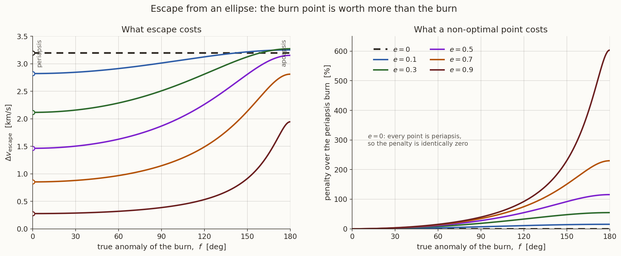
| \(e\) | \(\Delta v\) at periapsis | \(\Delta v\) at apoapsis | penalty |
|---|---|---|---|
| \(0\) | \(3.2001\) | \(3.2001\) | \(0\%\) |
| \(0.3\) | \(2.1172\) | \(3.2742\) | \(+55\%\) |
| \(0.5\) | \(1.4638\) | \(3.1540\) | \(+115\%\) |
| \(0.7\) | \(0.8527\) | \(2.8122\) | \(+230\%\) |
| \(0.9\) | \(0.2766\) | \(1.9461\) | \(\mathbf{+603\%}\) |
On a circle every point is periapsis and the choice is immaterial. On an eccentric orbit the choice is the dominant design variable: at \(e=0.9\) the wrong end costs seven times as much, because at periapsis the spacecraft already moves at \(97\%\) of the escape speed.
9.2 Does the cheap burn cost time?
Periapsis is the cheapest point but also the lowest, so one might expect to pay for the saving with a longer climb to the edge of the planet’s sphere of influence, at \(R_{\rm SOI}\approx9.25\times10^5\) km for the Earth (see the patched-conics note). It does not.
After a prograde burn at an apsis of radius \(q\), the escape orbit is a parabola with periapsis \(q\), so \(h=\sqrt{2\mu q}\) and
\[ v_r^2=v^2-\frac{h^2}{r^2}=\frac{2\mu}r-\frac{2\mu q}{r^2} \qquad\Longrightarrow\qquad v_r=\sqrt{\frac{2\mu}r}\sqrt{1-\frac qr}. \]
Integrate \(dt=dr/v_r\) from \(q\) to \(R\) (substitute \(u=r-q\)) and show that
\[ t(q\to R)=\frac23\sqrt{\frac{R-q}{2\mu}}\,(R+2q). \]
Then differentiate with respect to \(q\). For which \(q\) does raising the burn point shorten the trip?
What you should find
\[ \begin{aligned} t&=\frac1{\sqrt{2\mu}}\int_q^R\frac{r\,dr}{\sqrt{r-q}}=\frac1{\sqrt{2\mu}}\int_0^{R-q}\frac{u+q}{\sqrt u}\,du\\ &=\frac1{\sqrt{2\mu}}\left[\tfrac23u^{3/2}+2qu^{1/2}\right]_0^{R-q}=\frac23\sqrt{\frac{R-q}{2\mu}}(R+2q). \end{aligned} \]
\(dt/dq\propto3(R-2q)\), positive for \(q<R/2\). So raising the burn point lengthens the trip for every \(q<R/2=4.62\times10^5\) km, far beyond any practical apoapsis. A lower periapsis parabola carries more radial speed at every radius.The only real time cost of the periapsis burn is the coast down to periapsis from wherever the spacecraft happens to be, up to half a period. For orbits that share the LEO periapsis, that changes the verdict only at the two ends:
| \(e\) | verdict on burning at periapsis |
|---|---|
| \(<0.216\) | marginally slower, for a negligible saving: burn where you are |
| \(0.216\) to \(0.939\) | cheaper and faster: no trade-off |
| \(>0.939\) | still much cheaper, but half a period is now days: a genuine trade-off |
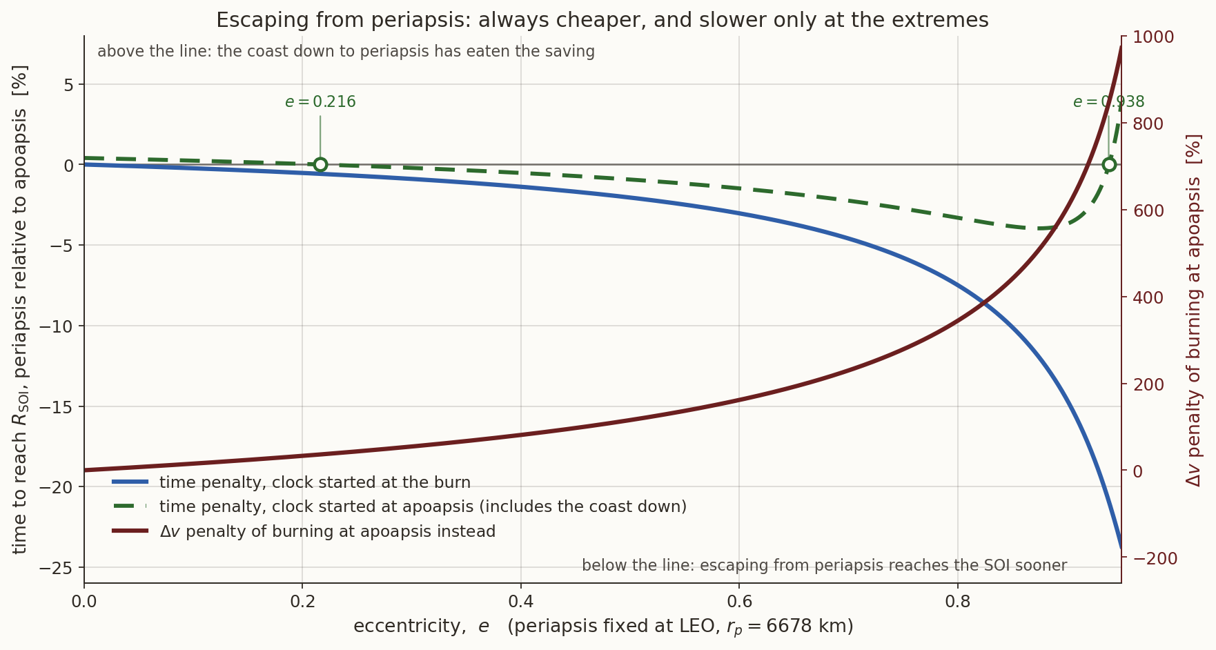
At \(e=0.9\) the periapsis burn saves \(1.67\) km/s and costs at most about a day of waiting; at \(e=0.95\) it saves \(1.34\) km/s and costs about three days. Against the rocket equation, the wait is almost always the better buy.
10 What these notes leave out
Everything above assumed impulsive burns, two bodies, and propulsion as the only force. Relaxing any one of these admits new manoeuvres, several of which current missions fly.
| assumption dropped | what appears | flown by, for example |
|---|---|---|
| impulsive burns | low-thrust spirals | all-electric GEO satellites, Dawn, BepiColombo |
| two bodies | gravity assists, low-energy transfers, libration-point orbits | Voyager, Hiten, GRAIL, JWST |
| propulsion only | aerobraking, aerocapture, solar sails | Mars Reconnaissance Orbiter, IKAROS |
Low thrust. An ion engine gives \(\sim0.1\) N for months, and the spacecraft spirals. For a slow quasi-circular spiral from speed \(v_1\) to \(v_2\) with a plane change \(\Delta i\) (in radians), Edelbaum’s classical approximation is
\[ \Delta v=\sqrt{v_1^2+v_2^2-2v_1v_2\cos\left(\frac\pi2\Delta i\right)}, \]
which for \(\Delta i=0\) is simply \(|v_1-v_2|\).
Compare LEO\(\to\)GEO with \(\Delta i=28.5^\circ\): impulsive with the optimal split (\(4.231\) km/s at \(I_{sp}=315\) s) against an Edelbaum spiral at \(I_{sp}=1800\) s. Use Equation 1 for the propellant fractions.
What you should find
Edelbaum: \(\sqrt{7.72576^2+3.07467^2-2(7.72576)(3.07467)\cos(0.7813)}=5.951\) km/s, \(41\%\) more than impulsive. But the propellant fractions are \(1-e^{-5.951/17.652}=28.6\%\) against \(1-e^{-4.231/3.089}=74.6\%\): less than half the propellant. Once the specific impulses differ, \(\Delta v\) alone is no longer the figure of merit. The price is time: months instead of hours.The atmosphere. Aerobraking dips the periapsis into the upper atmosphere and lets drag lower the apoapsis over many passes; Mars Reconnaissance Orbiter used it in 2006 to turn a \(35\)-hour capture orbit into a two-hour science orbit over about five months. Aerocapture would do the same in a single pass, converting an arriving hyperbola directly into a bound orbit. Both trade propellant for thermal protection and risk; recall from Section 3.3 that the atmosphere can supply only retrograde impulses.
A third body. A gravity assist rotates \(\mathbf v_\infty\) in the planet’s frame for free, which changes the speed in the Sun’s frame (see the two-body note). In the three-body problem, low-energy transfers reach the Moon or a libration point with far less \(\Delta v\) than patched conics predict; Hiten (1991) and GRAIL (2011) used them.
Station-keeping. Fighting perturbations, rather than changing orbit, has its own budget: a geostationary satellite spends about \(45\)–\(55\) m/s per year correcting the inclination drift caused by the Sun and Moon, and a few m/s per year holding its longitude.
Is a given transfer optimal? For impulsive transfers, Lawden’s primer vector theory answers this: along an optimal trajectory an adjoint vector \(\boldsymbol\lambda(t)\) satisfies \(|\boldsymbol\lambda|\le1\), with \(|\boldsymbol\lambda|=1\) exactly at the impulses and each \(\Delta\mathbf v_i\) parallel to \(\boldsymbol\lambda(t_i)\). If \(|\boldsymbol\lambda|>1\) somewhere between burns, adding an impulse there reduces the cost. This is how one shows, for example, that a given two-impulse transfer should have been bi-elliptic.
History: optimal manoeuvres. Derek Lawden introduced the primer vector in the 1950s and 1960s (Optimal Trajectories for Space Navigation, 1963). The bi-elliptic transfer was analysed by Ary Sternfeld in the 1930s and again, independently, in the late 1950s.
11 Summary
- An impulse buys energy at the rate \(v\,\Delta v\) (Equation 2) and turns the velocity at the cost \(2v\sin(\theta/2)\) (Equation 11). Energy favours large \(v\), turning favours small \(v\); most designs resolve that conflict. Propellant grows exponentially with \(\Delta v\) (Equation 1).
- Hohmann (Equation 3) is the cheapest two-impulse transfer between coplanar circles, for every radius ratio. Its cost peaks at \(R=15.58\).
- Between coaxial ellipses there are always two apsidal routes; with aligned apsides, periapsis of the inner orbit to apoapsis of the outer is always the cheaper. Crossing orbits allow a single impulse, which costs as a rotation of \(\mathbf v\).
- Bi-elliptic beats Hohmann for \(R>11.94\) with a large enough \(r_b\), and for any \(r_b>r_2\) when \(R>15.58\), the maximum of the Hohmann curve. A stopover (\(r_b<r_2\)) is always worse.
- Phasing: to catch up, burn retrograde; use more revolutions to save \(\Delta v\); on an ellipse, phase at periapsis.
- Apse rotation by a single radial impulse costs \(2v\sin\gamma\); above a crossover angle, go via a circle.
- Plane changes: at low speed, combined with a transfer burn, and shared between burns; or let \(J_2\) move the node for free.
- Escape is cheapest at periapsis, and the periapsis burn also reaches the sphere of influence sooner.
12 Exercises
- Moon transfer. Compute the Hohmann \(\Delta v\) and transfer time from LEO to a circular orbit of radius \(384\,400\) km (ignore the Moon’s gravity). Would a bi-elliptic transfer help?
- Going down. A satellite in GEO is to be de-orbited into an ellipse whose perigee is at \(100\) km altitude. What single burn does it need, and where? Compare with the cost of raising it \(300\) km into a graveyard orbit.
- Phasing in GEO. A geostationary satellite must move \(10^\circ\) east in longitude. Design a phasing manoeuvre that does it in \(5\) days. Which way does it burn first?
- Apse rotation. For an orbit with \(e=0.2\), find the crossover angle above which going via the circle is cheaper than a single radial impulse. How does it change with \(e\)?
- The best split. Repeat the optimal plane-change split for a launch from Sriharikota (\(\Delta i=13.7^\circ\), the latitude of the launch site, to GEO; starting from a \(300\) km parking orbit). How much does splitting save?
- Proof practice. In the Hohmann optimality proof, carry out the “similar inequality” of the case \(h>h_{\rm H}\) in full.
- Rocket equation. A spacecraft with \(I_{sp}=320\) s must deliver \(5\) km/s of \(\Delta v\). What fraction of its initial mass is left? What if the same \(\Delta v\) is shared between two stages of equal \(I_{sp}\) that each drop \(10\%\) of their initial mass as empty tanks?
All the numbers in this note, the worked examples and the task answers are checked by orbital-maneuvers-verify.py.