Chase Manoeuvres
Intercept and rendezvous between coplanar orbits
Outline
A chaser (1) on orbit \((a_1,e_1)\) must reach a target (2) on orbit \((a_2,e_2)\), using Lambert’s problem (\(p\)-iteration) far out and the Clohessy–Wiltshire equations close in.
- Part 0 defines intercept and rendezvous, and the two free parameters of every chase.
- Part I — both on the same orbit: the phasing manoeuvre.
- Part II — circular orbits, \(a_1<a_2\): wait for the Hohmann window, or pay to go now.
- Part III — elliptic orbits: the windows are no longer periodic.
- Part IV — the terminal phase, in the CW frame.
- Part V — the outer chaser, \(a_1>a_2\), by time reversal.
\(\mu_\oplus = 398600.4418\ \mathrm{km^3/s^2}\), \(R_\oplus = 6378.137\) km; orbits coplanar, motion prograde. Target in Parts I, II, IV: circular, \(420\) km (\(6798.137\) km); chaser in Part II: \(300\) km (\(6678.137\) km).
Part 0 — The Chase Problem
Intercept and rendezvous
At the meeting time \(t_f\):
| condition | burns | cost | |
|---|---|---|---|
| intercept | \(\mathbf r_1(t_f)=\mathbf r_2(t_f)\) | one, at departure | \(\Delta v_1\) |
| rendezvous | \(\mathbf r_1(t_f)=\mathbf r_2(t_f)\) and \(\mathbf v_1(t_f)=\mathbf v_2(t_f)\) | two | \(\Delta v_1+\Delta v_2\) |
An intercept arrives with a relative speed \(|\mathbf v_2-\mathbf v_1|\) — a collision, a fly-by, or a kinetic impactor. A rendezvous brakes that relative speed to zero.
For a given departure time and time of flight, both use the same transfer arc: the arc is fixed by where the chaser is and where the target will be. Rendezvous only adds the braking burn, and that burn equals the intercept’s arrival speed:
\[ \Delta v_{\rm rendezvous}=\Delta v_1+\underbrace{|\mathbf v_2(t_f)-\mathbf v_{\rm arc}(t_f)|}_{\text{intercept arrival speed}} . \]
The two problems share every arc but not the optimum: minimising \(\Delta v_1\) alone and minimising the sum pick different arcs.
Two free parameters
Every chase is a choice of
- the departure epoch \(t_0\) — how long we wait before the first burn;
- the time of flight \(\Delta t\) — how long the transfer takes.
Given \((t_0,\Delta t)\), Kepler’s equation places the chaser at \(\mathbf r_1(t_0)\) and the target at \(\mathbf r_2(t_0+\Delta t)\), and one Lambert solution gives the arc. Scanning the \((t_0,\Delta t)\) plane gives a porkchop plot; every design question in this deck is a walk on it.
For circular orbits the geometry depends on \(t_0\) only through the phase angle \(\theta\) — how far the target leads the chaser. It changes at the relative rate \(n_1-n_2\) and repeats after the synodic period
\[ T_{\rm syn}=\frac{2\pi}{|n_1-n_2|} . \qquad(1)\]
Part I — Same Orbit: Phasing
The phasing manoeuvre
Chaser and target share a circular orbit of period \(T\); the target leads by \(\theta\). The chaser burns onto a phasing ellipse with period \(T_{ph}\), flies \(k\) revolutions and returns to the burn point just as the target arrives there:
\[ k\,T_{ph}=kT-\frac{\theta}{2\pi}T \quad\Longrightarrow\quad \boxed{\ T_{ph}=T\Big(1-\frac{\theta}{2\pi k}\Big)\ } \qquad(2)\]
(If the target trails by \(\theta\), replace \(-\theta\) by \(+\theta\): arrive late on a larger ellipse.)
Kepler’s third law gives \(a_{ph}=a\,(T_{ph}/T)^{2/3}\); vis-viva at the burn point gives
\[ \Delta v=\Big|\sqrt{\frac{\mu}{a}}-\sqrt{\mu\Big(\frac{2}{a}-\frac{1}{a_{ph}}\Big)}\Big| . \]
Rendezvous: two equal burns, \(2\Delta v\). Intercept: the first burn only — and since the chaser returns to the burn point at the same speed it left with, it meets the target at relative speed exactly \(\Delta v\).
Example 1 — closing a \(20^\circ\) gap at 420 km
Given \(a=6798.137\) km, \(T=5578.22\) s. The target leads by \(20^\circ\) (drop, arrive early) or trails by \(20^\circ\) (raise, arrive late).
| \(k\) | \(a_{ph}\) [km] | far-apsis altitude [km] | \(2\Delta v\) [m/s] | time [h] | |
|---|---|---|---|---|---|
| target ahead | \(1\) | \(6543.96\) | \(\mathbf{-88.3}\) | \(300.36\) | \(1.463\) |
| \(2\) | \(6671.66\) | \(167.0\) | \(145.86\) | \(3.013\) | |
| \(3\) | \(6713.95\) | \(251.6\) | \(\mathbf{96.32}\) | \(4.562\) | |
| \(6\) | \(6756.11\) | \(335.9\) | \(47.71\) | \(9.211\) | |
| target behind | \(1\) | \(7047.64\) | \(919.0\) | \(268.73\) | \(1.636\) |
| \(3\) | \(6881.81\) | \(587.3\) | \(92.82\) | \(4.735\) |
With one revolution the phasing ellipse hits the Earth; with two, its perigee at \(167\) km is too deep in the atmosphere. Three revolutions is the practical minimum.
Cost and constraint against \(k\)
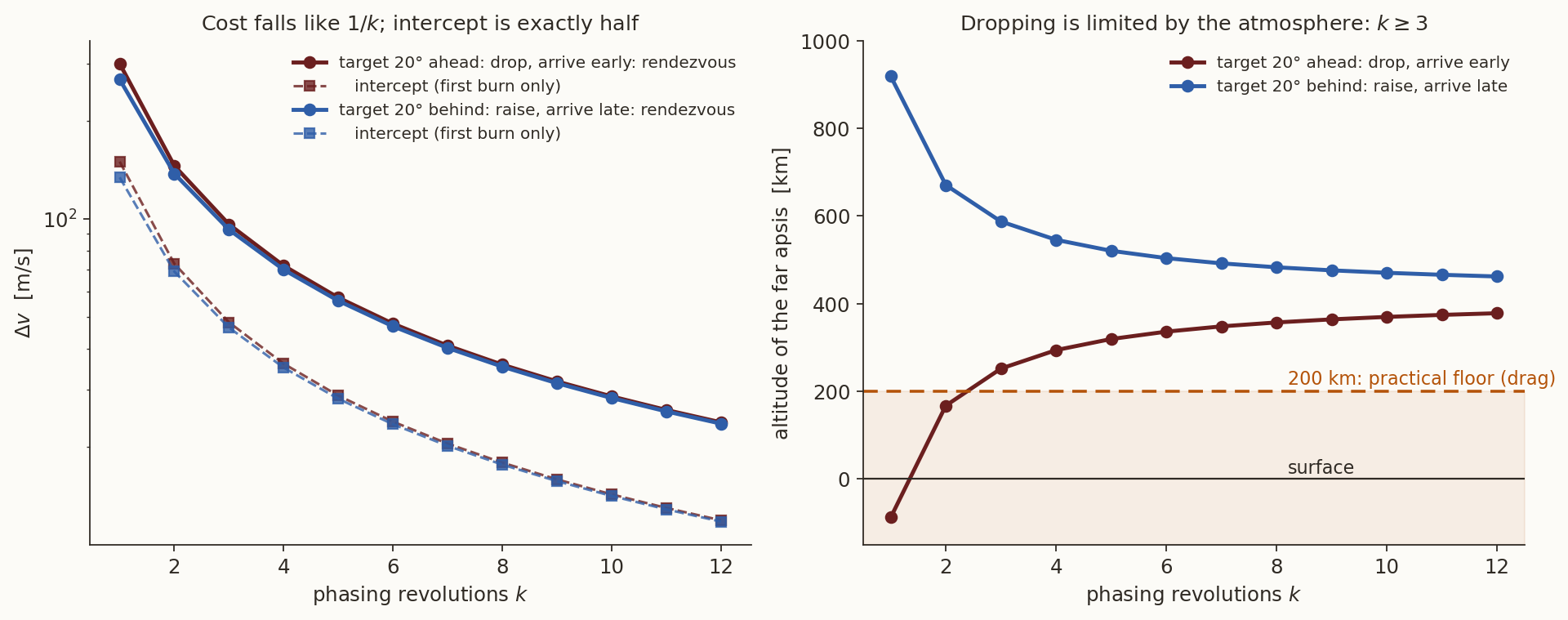
Figure 1: Left: the phasing cost falls essentially as \(1/k\), and the intercept costs exactly half the rendezvous. Right: the altitude of the phasing ellipse’s far apsis; dropping to catch a leading target is limited by the atmosphere, raising to wait for a trailing one is not.
Phasing on an elliptic orbit
On an ellipse the gap is naturally stated in true anomaly, but Equation 2 needs a time. Convert with Kepler’s equation.
Given \(a=10000\) km, \(e=0.3\), \(T=9952.01\) s. The chaser is at periapsis; the target is \(30^\circ\) behind, at \(f=-30^\circ\). The chaser must arrive late by the target’s time from \(f=-30^\circ\) to \(f=0\) — by symmetry, the time from \(0\) to \(30^\circ\):
\[ \tan\frac{E}{2}=\sqrt{\frac{1-e}{1+e}}\tan 15^\circ\ \Rightarrow\ E=0.388289, \qquad M=E-e\sin E=0.274707, \]
\[ \Delta t=\frac{M}{n}=\frac{0.274707}{6.313481\times10^{-4}}=435.11\ \mathrm s . \]
\(T_{ph}=T+\Delta t=10387.13\) s, \(a_{ph}=10289.39\) km, and a periapsis burn costs \(2\times64.904=\mathbf{129.81}\) m/s.
The same \(30^\circ\) at apoapsis takes \(1415.28\) s — \(3.3\) times longer — and costs \(703.17\) m/s. A fixed \(\Delta f\) is not a fixed \(\Delta t\); the burn point changes the required timing as well as the price.
Part II — Circular Orbits, \(a_1<a_2\)
The Hohmann rendezvous
The cheapest transfer between the circles is the Hohmann ellipse, flown in \(t_H=\pi\sqrt{a_t^3/\mu}\), \(a_t=\tfrac12(r_1+r_2)\). For the target to be at the meeting point, it must lead the chaser at the first burn by the lead angle
\[ \boxed{\ \theta^*=\pi-n_2\,t_H\ } \qquad(3)\]
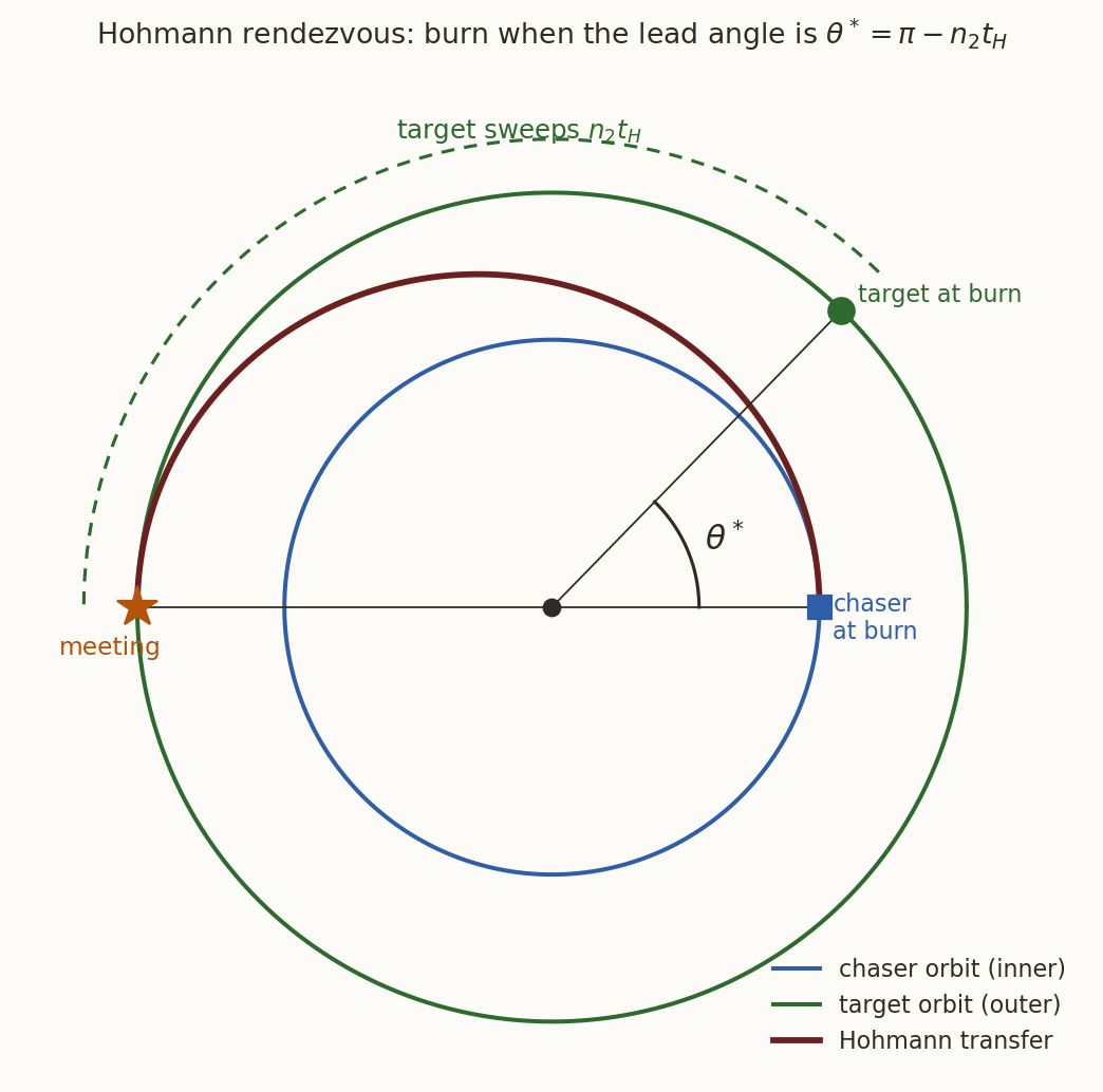
Figure 2: The chaser burns when the target leads by \(\theta^*\); during \(t_H\) the target sweeps \(n_2t_H\) and arrives at apoapsis with the chaser.
Example 2 — 300 km \(\to\) 420 km
\[ n_1=1.156874\times10^{-3},\quad n_2=1.126378\times10^{-3}\ \mathrm{rad/s}, \qquad t_H=2752.27\ \mathrm s=45.87\ \mathrm{min}. \]
\[ \Delta v_1=34.321,\qquad \Delta v_2=34.168,\qquad \Delta v_H=\mathbf{68.489}\ \mathrm{m/s}. \]
Lead angle. \(n_2t_H=177.622^\circ\), so \(\theta^*=\mathbf{2.378^\circ}\): the target must be barely ahead.
Waiting. The phase closes at \(n_1-n_2=6.290^\circ\)/h, and repeats every \(T_{\rm syn}=57.23\) h \(=2.38\) days (Equation 1). If the target now leads by \(\theta_0=40^\circ\),
\[ t_w=\frac{\theta_0-\theta^*}{n_1-n_2}=\frac{37.622^\circ}{6.290^\circ/\mathrm h}=\mathbf{5.98\ h}. \]
Had the target led by only \(\theta_0=0^\circ\) — the window just missed — the wait would be \(56.85\) h.
Waiting against paying
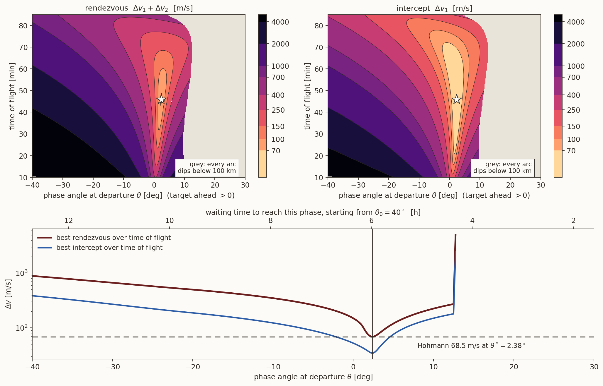
Figure 3: Top: porkchop over the phase angle at departure and the time of flight, rendezvous (left) and intercept (right). Only a narrow wedge around the Hohmann point (star) is cheap; grey means every zero-revolution arc dips below \(100\) km. Bottom: the best cost at each departure phase, and the waiting time needed to reach that phase from \(\theta_0=40^\circ\).
Reading the porkchop
| \(\theta\) | rendezvous [m/s] | intercept [m/s] |
|---|---|---|
| \(-20^\circ\) | \(499.7\) | \(187.5\) |
| \(-10^\circ\) | \(348.3\) | \(122.8\) |
| \(0^\circ\) | \(149.4\) | \(52.4\) |
| \(\mathbf{2.38^\circ}\) | \(\mathbf{68.8}\) | \(\mathbf{34.6}\) |
| \(5^\circ\) | \(119.6\) | \(75.9\) |
| \(10^\circ\) | \(224.6\) | \(149.7\) |
| \(>12.5^\circ\) | — | — |
- Leaving now from \(\theta_0=40^\circ\) is not merely expensive — every zero-revolution arc passes below \(100\) km. The chaser must wait (or phase over several revolutions).
- Each degree of phase costs \(9.54\) minutes of waiting. Leaving \(1\) h early (\(\theta\approx 8.7^\circ\)) roughly triples the bill.
- The best intercept is the Hohmann first burn, \(34.3\) m/s, arriving at \(34.2\) m/s: the tangential burn is the cheapest way to reach \(r_2\) at all.
- The intercept valley is wider: an intercept tolerates a timing error that a rendezvous pays for twice.
- In practice the wait is spent in a lower phasing orbit, with small height trims to tune the arrival — phasing and Hohmann combined.
Part III — Elliptic Orbits
The setting
Chaser \(a_1=6800\) km, \(e_1=0.02\) (\(r_p=6664\), \(r_a=6936\) km), \(T_1=1.5501\) h. Target \(a_2=10000\) km, \(e_2=0.3\) (\(r_p=7000\), \(r_a=13000\) km), \(T_2=2.7644\) h. The apse lines are aligned (\(\omega_1=\omega_2=0\)) and the orbits do not cross (\(r_{a,1}<r_{p,2}\)). At \(t=0\) the chaser is at periapsis and the target at \(M_2=90^\circ\).
Where is the target? Kepler’s equation, forward:
\[ M_2(t)=M_2(0)+n_2t \ \rightarrow\ E_2\ \ (\text{Newton on } M=E-e\sin E) \ \rightarrow\ f_2 \ \rightarrow\ \mathbf r_2(t),\ \mathbf v_2(t). \]
Now nothing is rotationally symmetric: the cost depends on \(t_0\) itself, not just on a phase.
Two Hohmann-like routes
With aligned apsides there are two apsis-to-apsis half-ellipses:
| route | radii [km] | \(t_H\) [h] | \(\Delta v_1\) | \(\Delta v_2\) | rendezvous | intercept |
|---|---|---|---|---|---|---|
| R1 peri \(\to\) apo | \(6664\to13000\) | \(1.3475\) | \(1082.17\) | \(74.10\) | \(\mathbf{1156.27}\) | \(1082.17\) |
| R2 apo \(\to\) peri | \(6936\to7000\) | \(0.8040\) | \(93.58\) | \(1075.12\) | \(1168.70\) | \(\mathbf{93.58}\) |
All speeds in m/s.
The rendezvous totals nearly tie; the intercept costs differ by a factor of \(11.6\). R2 does its cheap burn first, where the orbits nearly touch, and leaves the expensive matching to the braking burn — which an intercept never pays.
Timing. R1 departs at chaser periapsis (\(t_0=kT_1\)), R2 at apoapsis (\(t_0=(k+\tfrac12)T_1\)); the target must be at the arrival apsis \(t_H\) later. The two periods are incommensurate, so no departure ever times exactly. Within \(24\) h the closest calls are R2 at \(17.83\) h (\(106\) s early) and R1 at \(18.60\) h (\(335\) s early).
Example 3 — the elliptic porkchop
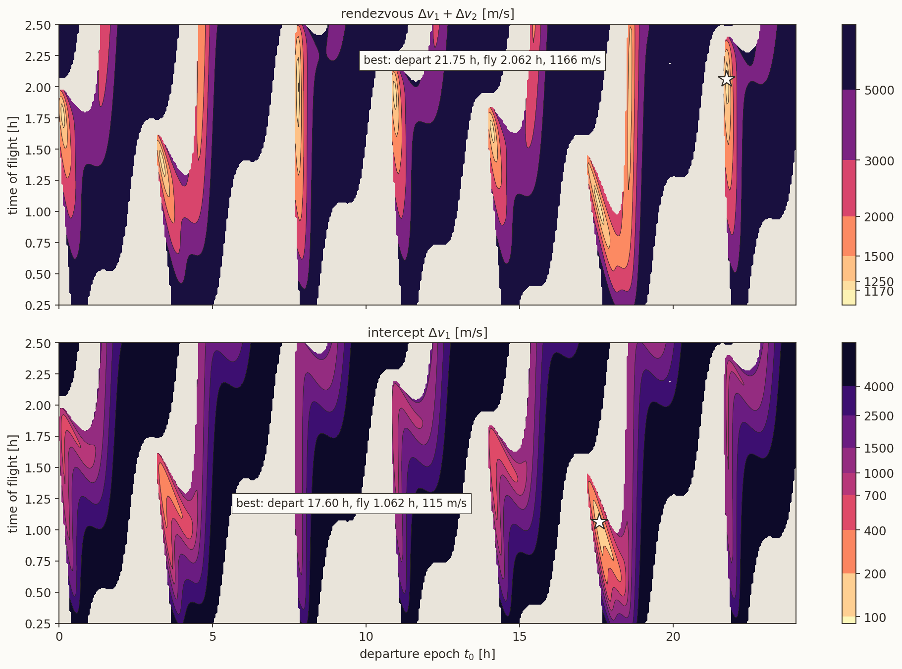
Figure 4: Porkchop for the elliptic chase over \(24\) h of departure epochs. Top: rendezvous; bottom: intercept. The cheap islands recur roughly every chaser period but their depth changes from one to the next, because the target’s position is not periodic in \(T_1\).
Example 3 — the optimum arcs
Best rendezvous (refined from the grid):
\[ t_0=21.757\ \mathrm h,\quad \Delta t=2.058\ \mathrm h,\quad \Delta v_1=952.50,\ \ \Delta v_2=211.90,\ \ \boxed{\ \Delta v=1164.40\ \mathrm{m/s}\ } \]
on an arc with \(p=8557.10\) km, \(e=0.2835\), sweeping \(265.7^\circ\) — not apsis to apsis, yet within \(0.7\%\) of R1.
Best intercept:
\[ t_0=17.623\ \mathrm h,\quad \Delta t=1.048\ \mathrm h,\quad \boxed{\ \Delta v_1=114.46\ \mathrm{m/s}\ },\quad \text{arrival speed } 1.087\ \mathrm{km/s} \]
near the R2 window (\(17.83\) h), paying \(21\) m/s above R2’s ideal \(93.6\) m/s to fix its timing.
The two optima are four hours apart and on different arcs. “Chase” is not one problem: say whether you must match velocity before you look for the window.
Part IV — The Terminal Phase
Switching to the CW frame
Once the chaser is within a few tens of kilometres, work in the target’s LVLH frame with the CW state transition matrix \(\mathbf\Phi(t)\) (the CW note). The chaser is at \(\mathbf r_0=(x_0,y_0)\) with velocity \(\mathbf v_0^-\); choose a transfer time \(t_f\).
Intercept — reach the origin:
\[ \mathbf 0=\mathbf\Phi_{rr}(t_f)\,\mathbf r_0+\mathbf\Phi_{rv}(t_f)\,\mathbf v_0^+ \quad\Longrightarrow\quad \boxed{\ \mathbf v_0^+=-\mathbf\Phi_{rv}^{-1}\mathbf\Phi_{rr}\,\mathbf r_0,\qquad \Delta\mathbf v_1=\mathbf v_0^+-\mathbf v_0^-\ } \]
Rendezvous — also cancel the arrival velocity:
\[ \mathbf v_f=\mathbf\Phi_{vr}\,\mathbf r_0+\mathbf\Phi_{vv}\,\mathbf v_0^+, \qquad \Delta\mathbf v_2=-\mathbf v_f . \]
\(\det\mathbf\Phi_{rv}=\big[8(1-\cos\tau)-3\tau\sin\tau\big]/n^{2}\), \(\tau=nt_f\), vanishes at \(\tau=2\pi k\) and at \(\tau=8.8387\) (\(t_f=1.4067\,T\)). At those transfer times no two-impulse solution exists for a general \(\mathbf r_0\).
Example 4 — 1 km below, 10 km behind
Given \(\mathbf r_0=(-1,\ -10)\) km on a co-circular drift, \(\mathbf v_0^-=(0,\ \tfrac32 n)\) km/s \(=(0,\ 1.690)\) m/s — closing at \(9.42\) km per orbit on its own.
| \(t_f\) | \(T/4\) | \(T/2\) | \(3T/4\) | \(5T/4\) | \(3T/2\) |
|---|---|---|---|---|---|
| minutes | \(23.2\) | \(46.5\) | \(69.7\) | \(116.2\) | \(139.5\) |
| intercept \(\Delta v_1\) [m/s] | \(6.401\) | \(2.171\) | \(1.222\) | \(1.158\) | \(0.872\) |
| arrival speed \(=\Delta v_2\) [m/s] | \(7.154\) | \(2.171\) | \(0.618\) | \(0.580\) | \(0.872\) |
| rendezvous [m/s] | \(13.555\) | \(4.342\) | \(\mathbf{1.840}\) | \(\mathbf{1.738}\) | \(1.744\) |
Cross-check with Lambert. Solving the same geometry exactly by \(p\)-iteration gives \((\Delta v_1,\Delta v_2)=(6.401,\ 7.156)\), \((2.171,\ 2.174)\), \((1.219,\ 0.618)\) m/s at \(T/4\), \(T/2\), \(3T/4\) — agreement to better than \(0.3\%\). The \(T/2\) arc sweeps \(180.08^\circ\), right at Lambert’s pinch; CW has no difficulty there. Its own singularities are elsewhere.
Trajectories and cost
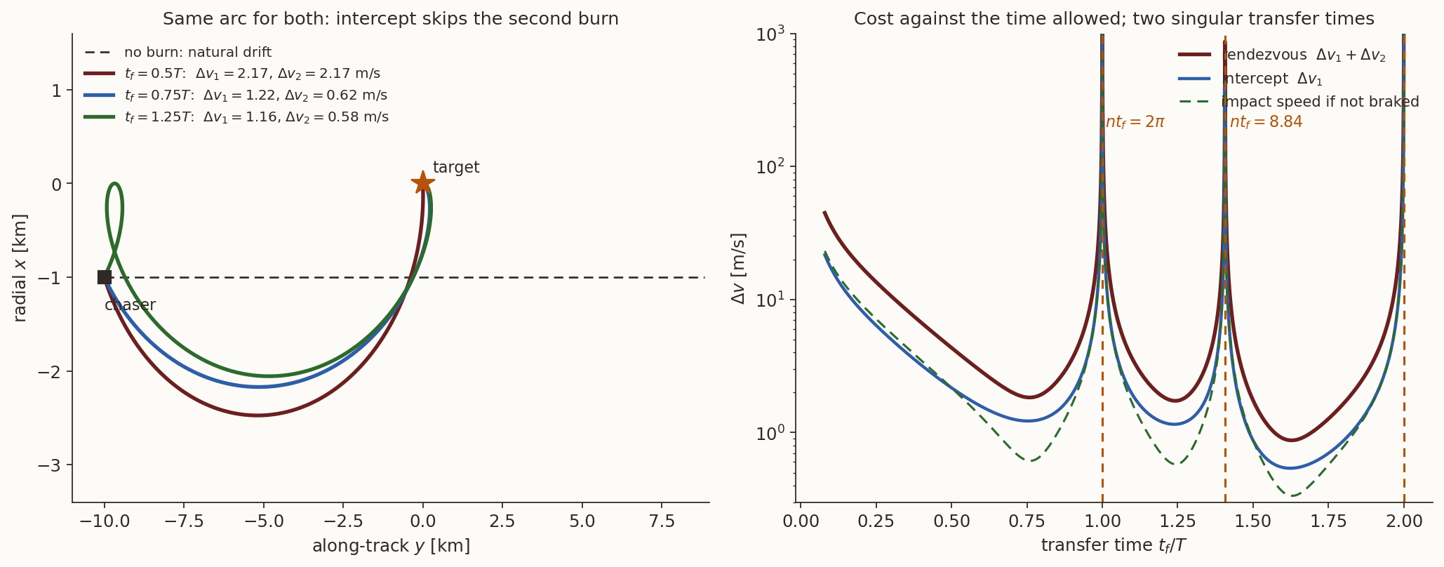
Figure 5: Left: CW transfers from \((-1,-10)\) km for three transfer times; intercept and rendezvous fly the same arc, and differ only in the braking burn at the origin. Right: cost against the transfer time, with the singular times \(nt_f=2\pi\), \(8.84\) and \(4\pi\) marked.
Part V — The Outer Chaser, \(a_1>a_2\)
Time reversal
Gravity is conservative and time-independent, so if \(\mathbf r(t)\) is a trajectory then so is \(\mathbf r(-t)\), flown with every velocity reversed. Reflecting the orbit plane restores prograde motion. Applied to a transfer from orbit 1 to orbit 2:
- the arc becomes a transfer from orbit 2 to orbit 1, with the same time of flight;
- the departure burn becomes the arrival burn and vice versa.
Rendezvous maps to rendezvous with \(\Delta v_1\leftrightarrow\Delta v_2\): the same total. Every rendezvous result for \(a_1<a_2\) carries over to \(a_1>a_2\) unchanged.
Intercept does not. The reversed intercept pays at departure what the forward one arrived with:
\[ \Delta v_{\rm intercept}^{\,2\to1}=\text{arrival speed}^{\,1\to2}, \qquad \text{arrival speed}^{\,2\to1}=\Delta v_{\rm intercept}^{\,1\to2}. \]
The asymmetry, in numbers
Hohmann intercepts between circles:
| orbits | inner \(\to\) outer intercept | its arrival speed | outer \(\to\) inner intercept | its arrival speed |
|---|---|---|---|---|
| \(300\leftrightarrow420\) km | \(34.32\) m/s | \(34.17\) m/s | \(34.17\) m/s | \(34.32\) m/s |
| LEO \(\leftrightarrow\) GEO | \(2425.7\) m/s | \(1466.8\) m/s | \(1466.8\) m/s | \(2425.7\) m/s |
Nearby orbits hide the asymmetry (\(0.4\%\)); widely separated ones expose it (a factor of \(1.65\)).
The window reverses too. For the outer chaser the target moves faster, so \(\theta^*=\pi-n_{\rm inner}t_H\) is negative: at \(420\to300\) km the target must trail by \(2.431^\circ\).
Summary
- Intercept matches position; rendezvous matches position and velocity. For given \((t_0,\Delta t)\) they share the arc; rendezvous adds the arrival speed as a braking burn.
- Same orbit: phasing, \(T_{ph}=T(1\mp\theta/2\pi k)\). Cost \(\propto 1/k\); the atmosphere limits how far one may drop. On an ellipse, convert \(\Delta f\) to \(\Delta t\) by Kepler’s equation.
- Circular orbits: burn at the lead angle \(\theta^*=\pi-n_2t_H\), repeating every \(T_{\rm syn}\). Leaving off-window is expensive or impossible; waiting is cheap.
- Elliptic orbits: windows are not periodic; the porkchop is the design tool, and the intercept and rendezvous optima can be hours apart.
- Close in: CW targeting, \(\mathbf v_0^+=-\mathbf\Phi_{rv}^{-1}\mathbf\Phi_{rr}\mathbf r_0\), agrees with Lambert and avoids its \(180^\circ\) pinch — but has singular times of its own.
- Outer chaser: time reversal preserves rendezvous costs and swaps intercept cost with arrival speed.

SFM, IIST 2026