Notation and Constants
The symbols and numbers shared by all the orbital mechanics notes
All the notes use the symbols below. A note that needs a symbol for something else says so where it does, and keeps the meaning local. The last column gives the symbol that Curtis’s Orbital Mechanics for Engineering Students (the course textbook) uses, where it differs; a dash means no counterpart is listed. Each note’s opening section says which other notes it builds on; the study plan gives the order.
Orbits and their integrals
| Symbol | Meaning | First defined in | Curtis |
|---|---|---|---|
| \(\mu=Gm\) | gravitational parameter of the attracting body; \(\mu_\odot\), \(\mu_\oplus\) for the Sun and the Earth, \(\mu_{\rm Moon}\), \(\mu_{\rm Mars}\) and so on spelled out | N-body | \(\mu\) |
| \(\mathbf r\), \(\mathbf v\); \(r\), \(v\) | position and velocity relative to the attracting body, and their lengths | Two-body | same |
| \(\mathbf h=\mathbf r\times\mathbf v\), \(h\) | specific angular momentum | Two-body | same |
| \(\varepsilon=\frac{v^2}{2}-\frac\mu r\) | specific energy | Two-body | same |
| \(\mathbf e\), \(e\) | eccentricity vector and eccentricity | Two-body | same |
| \(p=h^2/\mu\) | semi-latus rectum | Two-body | \(h^2/\mu\) |
| \(a=-\mu/(2\varepsilon)\) | semi-major axis, negative on a hyperbola | Two-body | same |
| \(f\) | true anomaly | Two-body | \(\theta\) |
| \(\gamma\) | flight-path angle, from the local horizontal | Two-body | same |
| \(v_r\), \(v_\perp\) | radial and transverse parts of \(\mathbf v\) | Two-body | same |
| \(E\); \(M=E-e\sin E\); \(n=\sqrt{\mu/a^3}\) | eccentric anomaly, mean anomaly, mean motion | Two-body | \(E\); \(M_e\); \(n\) |
| \(D=\tan\frac f2\); \(M_p=D+\frac13D^3\) | parabolic anomaly and its mean anomaly | Two-body | \(M_p=\frac12\tan\frac\theta2+\frac16\tan^3\frac\theta2\), half of ours |
| \(H\); \(M_h=e\sinh H-H\) | hyperbolic anomaly and its mean anomaly | Two-body | \(F\); \(M_h\) |
| \(v_\infty\); \(C_3=v_\infty^2\) | hyperbolic excess speed; characteristic energy | Two-body | same |
| \(f_\infty=\arccos(-1/e)\); \(\delta=2\arcsin(1/e)\) | asymptote angle; turning angle | Two-body | \(\theta_\infty\); \(\delta\) |
| \(b=\lvert a\rvert\sqrt{e^2-1}\) | aiming radius (impact parameter), written \(\Delta\) in the two-body note | Two-body | \(\Delta\) |
| \(t_p\) | time of periapsis passage | Two-body | same |
Frames, angles and matrices
| Symbol | Meaning | First defined in | Curtis |
|---|---|---|---|
| \(\hat{\mathbf I},\hat{\mathbf J},\hat{\mathbf K}\) | inertial (geocentric equatorial) axes; \(\hat{\mathbf K}\) along the pole | Orbital elements | same |
| \(\hat{\mathbf p},\hat{\mathbf q},\hat{\mathbf w}\) | perifocal axes: towards periapsis, \(90^\circ\) ahead, along \(\mathbf h\) | Perifocal | same |
| \(i\), \(\Omega\), \(\omega\) | inclination, right ascension (or longitude) of the ascending node, argument of periapsis | Perifocal | same |
| \(u=\omega+f\) | argument of latitude | Perifocal | same |
| \(\varpi\), \(\lambda\) | longitude of periapsis, true longitude (for equatorial orbits) | Orbital elements | same |
| \(\mathbf n=\hat{\mathbf K}\times\mathbf h\) | node vector, along the ascending node | Orbital elements | \(\mathbf N\) |
| \(\mathbf R_1(\theta)\), \(\mathbf R_3(\theta)\) | active rotations by \(\theta\) about the first and third axes | Perifocal | Curtis uses frame rotations, the transposes |
| \(\mathbf Q=\mathbf R_3(\Omega)\mathbf R_1(i)\mathbf R_3(\omega)\) | perifocal components to inertial ones | Perifocal | Curtis tabulates the inverse map, geocentric to perifocal, which is \(\mathbf Q^{\mathsf T}\) |
| \(\theta_G\) | Greenwich sidereal angle | Time | — |
| \(\varphi\), \(\lambda\) | geodetic latitude and east longitude of a station or a point on the Earth (\(\varphi_{gc}\) is the geocentric latitude) | Ground tracks, Topocentric | — |
| \(\hat{\mathbf S},\hat{\mathbf E},\hat{\mathbf Z}\) | topocentric axes: south, east, zenith | Topocentric | — |
| \(\rho\), \(A\), \(\varepsilon\) | range, azimuth (from north, clockwise) and elevation of a satellite seen from a station | Topocentric | \(\rho\), \(A\), \(a\) (elevation) |
| \(\alpha\), \(\delta\) | (topocentric) right ascension and declination of a direction | Topocentric | same |
The orbit-following frame has three names in the notes, and is one frame. Its axes point radially outwards, along the transverse direction (along the velocity only on a circular orbit) and along \(\mathbf h\):
| Note | Name | Unit vectors | Coordinates |
|---|---|---|---|
| Two-body, perifocal | polar basis | \(\hat{\mathbf r},\hat{\boldsymbol\theta},\hat{\mathbf h}\) | \(r\), \(f\) |
| CW equations, chase | LVLH (local vertical, local horizontal) | \(\hat{\mathbf i},\hat{\mathbf j},\hat{\mathbf k}\) | \(x\), \(y\), \(z\) |
| Gauss equations | RSW | \(\hat{\mathbf R},\hat{\mathbf S},\hat{\mathbf W}\) | force components \(a_R\), \(a_S\), \(a_W\) |
Other books order these axes differently (NASA’s LVLH, for example, puts \(x\) along the velocity and \(z\) towards the Earth), which permutes the rows of every matrix written in them.
The five frames and the matrices between them
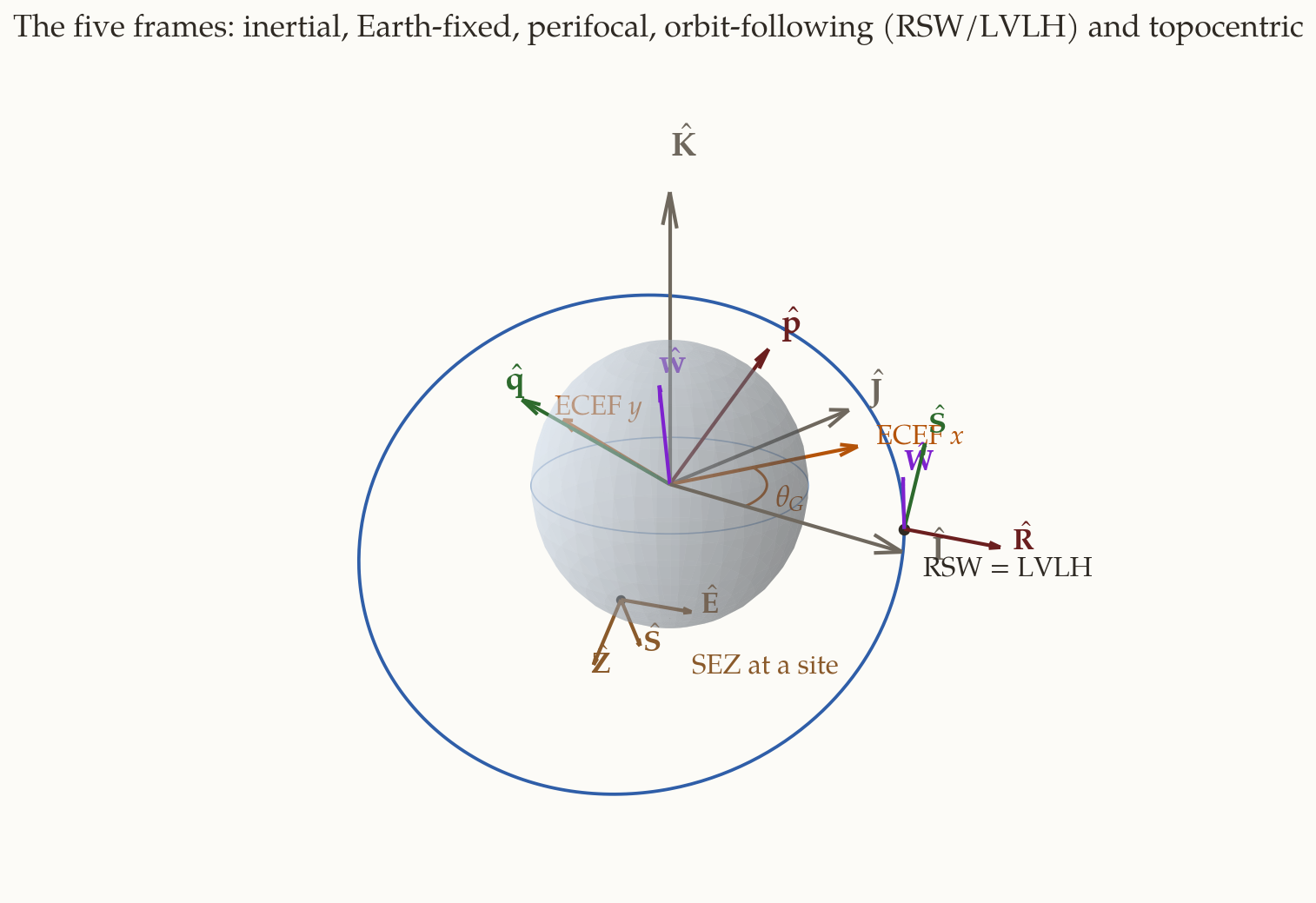
Each matrix below takes the components of a vector in the first frame to its components in the second (all rotations active, as in the perifocal note).
| From | To | Matrix | Where |
|---|---|---|---|
| perifocal | inertial | \(\mathbf Q=\mathbf R_3(\Omega)\mathbf R_1(i)\mathbf R_3(\omega)\) | Perifocal |
| orbit-following (RSW) | inertial | \(\mathbf R_3(\Omega)\mathbf R_1(i)\mathbf R_3(u)\), with \(u=\omega+f\) | Gauss equations |
| inertial | Earth-fixed | \(\mathbf R_3(-\theta_G)\) | Ground tracks, Time for \(\theta_G\) |
| Earth-fixed | topocentric (SEZ), at geodetic latitude \(\varphi\) and east longitude \(\lambda\) | rows \(\hat{\mathbf S},\hat{\mathbf E},\hat{\mathbf Z}\) written in ECEF components: \((\sin\varphi\cos\lambda,\ \sin\varphi\sin\lambda,\ -\cos\varphi)\), \((-\sin\lambda,\ \cos\lambda,\ 0)\), \((\cos\varphi\cos\lambda,\ \cos\varphi\sin\lambda,\ \sin\varphi)\) | Topocentric |
The reverse maps are the transposes. The angles and ranges measured in the topocentric frame are the input of orbit determination; its symbols are listed below.
Transfers, targeting and perturbations
| Symbol | Meaning | First defined in | Curtis |
|---|---|---|---|
| \(\Delta v\); \(v_e=I_{sp}g_0\) | velocity change; exhaust speed | Impulsive model | same |
| \(r_{\rm SOI}\) | radius of a sphere of influence | Patched conics | same |
| \(\Delta\theta\) | transfer angle between two position vectors | Lambert | same |
| \(F,G,\dot F,\dot G\) | Lagrange coefficients: \(\mathbf r=F\mathbf r_0+G\mathbf v_0\), \(\mathbf v=\dot F\mathbf r_0+\dot G\mathbf v_0\) | Perifocal | \(f,g,\dot f,\dot g\) |
| \(\chi\); \(z=\alpha\chi^2\); \(C(z)\), \(S(z)\) | universal anomaly, its square in units of the orbit, Stumpff functions (\(\alpha=1/a\)) | Universal variables | same |
| \(n\) (in the CW note) | mean motion of the target’s circular orbit | CW equations | same |
| \(\boldsymbol\rho\) | position of the chaser relative to the target | CW equations | — |
| \(J_2\); \(R_\oplus\) | Earth’s oblateness coefficient; its equatorial radius | Earth’s gravity | \(J_2\); \(R\) |
| \(\mathbf a_d\) | perturbing (disturbing) acceleration | Gauss equations | \(\mathbf p\) |
| \(\mu=m_2/(m_1+m_2)\); \(C\); \(\Omega\) | mass parameter, Jacobi constant and pseudo-potential of the restricted three-body problem (local to that note) | Restricted three-body | — |
| \(L_1,\dots,L_5\) | Lagrange (libration) points | Restricted three-body | same |
Observations and orbit determination
The orbit-determination note takes its station, azimuth, elevation, right ascension and declination from the topocentric note (rows above) and adds these.
| Symbol | Meaning | First defined in | Curtis |
|---|---|---|---|
| \(t_1,t_2,t_3\); \(\tau_1=t_1-t_2\), \(\tau_3=t_3-t_2\), \(\tau=t_3-t_1\) | the three observation epochs and the intervals between them; \(\tau_1<0<\tau_3\) | Orbit determination | — |
| \(\mathbf R_i\), \(\dot{\mathbf R}_i\), \(\ddot{\mathbf R}_i\) | inertial position, velocity and acceleration of the station at \(t_i\); \(\mathbf R_i=\mathbf R_3(\theta_G(t_i))\,\mathbf r_{\rm site}\) | Orbit determination | — |
| \(\rho_i\), \(\mathbf L_i\) | range and unit line of sight (the \(\hat{\boldsymbol\rho}\) of the topocentric note), \(\mathbf r_i=\mathbf R_i+\rho_i\mathbf L_i\), with \(\mathbf L_i\) built from \(\alpha_i,\delta_i\) | Orbit determination, Topocentric | — |
| \(\mathbf D\), \(\mathbf N\), \(\mathbf S\) | Gibbs’s vectors: \(\mathbf D=\mathbf r_1\times\mathbf r_2+\mathbf r_2\times\mathbf r_3+\mathbf r_3\times\mathbf r_1\) and \(\mathbf N=r_1\,\mathbf r_2\times\mathbf r_3+r_2\,\mathbf r_3\times\mathbf r_1+r_3\,\mathbf r_1\times\mathbf r_2\) along \(\mathbf h\), with \(p=N/D\); \(\mathbf S=\mathbf r_1(r_2-r_3)+\mathbf r_2(r_3-r_1)+\mathbf r_3(r_1-r_2)\), perpendicular to \(\mathbf e\), with \(\mathbf e=\mathbf S\times\mathbf D/D^2\) | Orbit determination | — |
| \(D_0=\mathbf L_1\cdot(\mathbf L_2\times\mathbf L_3)\) | triple product of the three lines of sight; the determinant of Gauss’s linear system for the ranges, and a measure of how well the pass is placed | Orbit determination | — |
| \(c_1,c_3\) | weights in \(\mathbf r_2=c_1\mathbf r_1+c_3\mathbf r_3\) (Gauss), built from the Lagrange coefficients \(F_i,G_i\) of the interval from \(t_2\) to \(t_i\) | Orbit determination | — |
| \(\mathbf x\); \(\mathsf H\); \(\mathsf P=\sigma^2(\mathsf H^{\mathsf T}\mathsf H)^{-1}\) | least squares: the state at the reference epoch; the matrix \(\partial\mathbf h/\partial\mathbf x\) of the predicted angles; the covariance of \(\mathbf x\), with \(\sigma\) the standard deviation of one angle | Orbit determination | — |
Some of these letters have another meaning elsewhere on this page; the orbit-determination note uses the meaning given here. \(\mathbf R_i\) with an index is the position of the station, while \(\mathbf R_1(\theta)\), \(\mathbf R_3(\theta)\) with an argument are rotations, and \(\hat{\mathbf R}\) is the radial axis. \(\mathbf S\) (bold, no hat) is Gibbs’s vector, not the south axis \(\hat{\mathbf S}\). \(D\), \(D_0\), \(D_1\) and \(D_{ij}\) are determinants and triple products, not the parabolic anomaly \(D=\tan\frac f2\). The upright \(\mathsf H\) is a matrix, not the hyperbolic anomaly \(H\), and \(\mathsf P\) is not \(p\). And \(\alpha\) and \(\delta\) are right ascension and declination, never \(1/a\) or the turning angle.
Constants
The notes use these values. Some quote \(\mu_\oplus\) rounded to \(398\,600\) km\(^3\)/s\(^2\), as Curtis does; the difference is below the accuracy of any number they quote.
| Quantity | Value |
|---|---|
| \(\mu_\oplus\) | \(398\,600.4418\) km\(^3\)/s\(^2\) |
| \(R_\oplus\) (equatorial, WGS-84) | \(6378.137\) km |
| \(J_2\) (Earth) | \(1.08263\times10^{-3}\) |
| \(\omega_\oplus\) (rotation against the stars) | \(7.2921151\times10^{-5}\) rad/s |
| sidereal day | \(86\,164.0905\) s \(=23.9345\) h |
| \(\mu_\odot\) | \(1.327\,124\,400\,18\times10^{11}\) km\(^3\)/s\(^2\) |
| \(R_\odot\) | \(6.957\times10^{5}\) km |
| astronomical unit | \(1.495\,978\,707\times10^{8}\) km |
| \(\mu_{\rm Moon}\); \(R_{\rm Moon}\); Earth–Moon distance | \(4902.8\) km\(^3\)/s\(^2\); \(1737.4\) km; \(384\,400\) km |
| \(\mu_{\rm Mars}\); \(R_{\rm Mars}\); \(a_{\rm Mars}\) | \(42\,828.37\) km\(^3\)/s\(^2\); \(3396.2\) km; \(1.52368\) AU |
| \(\mu_J\); \(R_J\); \(a_J\) | \(1.266\,865\,34\times10^{8}\) km\(^3\)/s\(^2\); \(71\,492\) km; \(5.2026\) AU |
| \(g_0\) (for \(I_{sp}\)) | \(9.80665\) m/s\(^2\) |