Topocentric Frames and Observations
Where we are going
Everything so far was computed at the centre of the Earth. But nobody measures a satellite from the centre of the Earth. A radar on the ground measures how far the satellite is (range), and in which direction (azimuth and elevation), and an optical telescope measures only the direction (as right ascension and declination). A radio receiver measures how fast the range is changing, through the Doppler shift. All of these are quantities in a frame attached to the observer, the topocentric frame, and the only way to use them in the rest of astrodynamics is to know the observer’s position and orientation precisely and to convert between the frame of the observer and the inertial frame of the orbit. That conversion is this note.
The required background is the two-body problem, the orbital elements (especially the algorithm from a state vector to the elements), the active rotation matrices of the perifocal note, and the Greenwich sidereal angle and the Earth’s rotation rate of the time note. The sub-satellite point and the footprint of a satellite are in the ground-tracks note; this note looks at the same geometry from the other end. The next step in the course, preliminary orbit determination (Gibbs, Lambert-based and angles-only methods), builds directly on the observations defined here, and this note stops where it begins. As in the other notes, a blue Try it box asks you to do a small calculation before reading on, and a green Check yourself box asks a short question; each has a hidden answer.
Symbols and constants shared by all the notes are collected on the notation page; the study plan gives the order in which to read the notes. In this note \(\varphi\) is the geodetic latitude (the one on maps and GPS receivers) and \(\lambda\) the east longitude of the site, \(\varphi_{gc}\) the geocentric latitude, \(A\) the azimuth, and \(\varepsilon\) the elevation (the only use of \(\varepsilon\) in this note; it is not an energy).
1 The observer on the ellipsoid
1.1 Two kinds of latitude
The Earth is flattened by its rotation (the gravity note explains why), and the surface that surveyors and GPS use is a reference ellipsoid, a surface of revolution with equatorial radius \(a\) and flattening \(f\). The standard one is WGS 84 (National Imagery and Mapping Agency 2000):
TODO: This diagram is wrong. Correct it. Define both angles at the equatorial plane.
\[ a=6378.137\ \text{km},\qquad f=\frac1{298.257\,223\,563},\qquad e^{2}=f(2-f)=0.006\,694\,380 . \]
Here \(e\) is the eccentricity of the ellipsoid (not of an orbit). Two latitudes describe the direction of a point.
- The geocentric latitude \(\varphi_{gc}\) is the angle between the equatorial plane and the line from the Earth’s centre to the point. It is the latitude used for \(\sin\varphi_{gc}=z/r\) in the gravity and ground-track notes.
- The geodetic latitude \(\varphi\) is the angle between the equatorial plane and the normal to the ellipsoid at the point (Figure 1). It is the latitude of maps and of GPS, and, since the normal is what a plumb line (or a level) follows, it is the latitude that fixes which way is up for an observer.
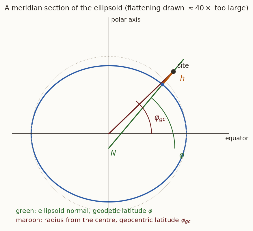
They agree at the equator and at the poles and differ in between, by at most
\[ \varphi-\varphi_{gc}\le0.192^\circ=11.5'\qquad\text{at }\varphi\approx45.1^\circ, \]
which is \(21\) km along the ground. That sounds small, but we will see that using the wrong one in the wrong place tilts the local vertical by that amount, and an elevation error of \(0.19^\circ\) at \(1000\) km range is \(3.4\) km.
If I put a spirit level normal to the line joining the a point on an ellipsoidal earth (with constant gravity) then the bubble will be in the center. True/False? What happens for real Earth? In other words, we are asking the question if the gravitational field be locally perpendicular to the Earth surface at point?
1.2 The site vector
Take a point on the surface at geodetic latitude \(\varphi\). In the meridian plane, let its distance from the polar axis be \(\varrho\) and its height above the equatorial plane \(z\). The ellipse is \(\varrho^{2}/a^{2}+z^{2}/b^{2}=1\) with \(b^{2}=a^{2}(1-e^{2})\). Its normal at the point points along the gradient \((\varrho/a^{2},\ z/b^{2})\), and that direction is \((\cos\varphi,\sin\varphi)\) by definition of geodetic latitude, so
\[ \frac z\varrho=\frac{b^{2}}{a^{2}}\tan\varphi=(1-e^{2})\tan\varphi . \]
Putting this into the ellipse equation,
\[ \varrho^{2}\left[\frac1{a^{2}}+\frac{(1-e^{2})^{2}\tan^{2}\varphi}{a^{2}(1-e^{2})}\right]=1 \ \Longrightarrow\ \varrho=\frac{a\cos\varphi}{\sqrt{1-e^{2}\sin^{2}\varphi}}\equiv N\cos\varphi, \qquad z=N(1-e^{2})\sin\varphi, \]
where
\[ N(\varphi)=\frac{a}{\sqrt{1-e^{2}\sin^{2}\varphi}} \tag{1}\]
is the length of the normal from the surface to the polar axis (the prime vertical radius of curvature). A point a height \(h\) above the surface along the normal is \(h\,(\cos\varphi\cos\lambda,\ \cos\varphi\sin\lambda,\ \sin\varphi)\) further out, so in Earth-fixed (ECEF) components
\[ \boxed{\ \mathbf r_{\rm site}=\begin{bmatrix}(N+h)\cos\varphi\cos\lambda\\ (N+h)\cos\varphi\sin\lambda\\ \bigl(N(1-e^{2})+h\bigr)\sin\varphi\end{bmatrix}\ } \tag{2}\]
and the geocentric latitude of the site is \(\varphi_{gc}=\operatorname{atan2}(z_{\rm site},\sqrt{x_{\rm site}^{2}+y_{\rm site}^{2}})\).
A station near Bengaluru is at geodetic latitude \(12.97^\circ\)N, longitude \(77.59^\circ\)E, height \(0.92\) km. Find \(N\), the site vector in ECEF, and the geocentric latitude.
What you should find
\(N=6379.2127\) km. \(\mathbf r_{\rm site}=(1336.147,\ 6072.091,\ 1422.378)\) km, with \(|\mathbf r_{\rm site}|=6377.99\) km. The geocentric latitude is \(12.886^\circ\), which is \(5.03'\) less than the geodetic one.Where on the Earth is \(\mathbf r_{\rm site}\) simply \((a+h)\) times a unit vector? Where is the flattening felt most?
Answer
At the equator, \(N=a\), \(z=0\) and \(\mathbf r_{\rm site}=(a+h)(\cos\lambda,\sin\lambda,0)\); at the poles, \(N=a/\sqrt{1-e^2}=a^{2}/b\) and \(z=(a^{2}/b)(1-e^{2})+h=b+h\), so \(\mathbf r_{\rm site}=(0,0,b+h)\), the shorter polar radius \(b=6356.752\) km. The direction of the vertical differs from the direction of the radius most at mid-latitudes (\(45^\circ\)), by the \(0.192^\circ\) above.History: reference ellipsoids. WGS 84 is the reference ellipsoid of GPS. Its two defining numbers are the equatorial radius, \(6\,378\,137\) m exactly, and the flattening, \(1/298.257\,223\,563\). Older national surveys used other ellipsoids, chosen to fit one region well, and the differences in the position of a point can reach hundreds of metres. For orbit work the difference between geodetic and geocentric latitude matters far more than the difference between ellipsoids.
2 The topocentric frame
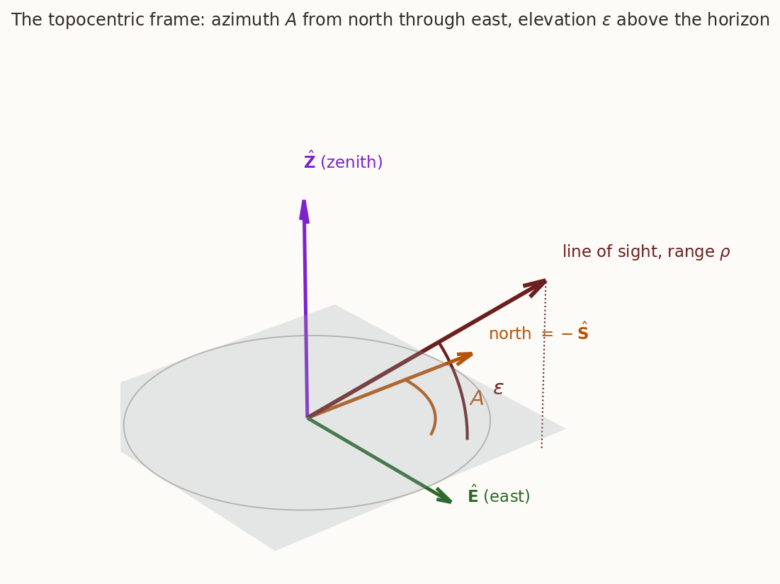
An observer needs three directions: up, east and north. The topocentric horizon frame, or SEZ frame, has its origin at the site and its axes along
- \(\hat{\mathbf Z}\), the local vertical (the outward normal to the ellipsoid, the zenith direction),
- \(\hat{\mathbf E}\), due east (the direction in which the longitude increases),
- \(\hat{\mathbf S}\), due south, chosen so that \((\hat{\mathbf S},\hat{\mathbf E},\hat{\mathbf Z})\) is right-handed, \(\hat{\mathbf S}\times\hat{\mathbf E}=\hat{\mathbf Z}\).
(Many books use the equivalent east-north-up, ENU, frame, with \(\hat{\mathbf N}=-\hat{\mathbf S}\) in place of \(\hat{\mathbf S}\). The two differ only by the sign of one axis, and by the order of the rows of the matrix below.) Figure 2 draws the frame.
In ECEF components, \(\hat{\mathbf Z}\) is the outward ellipsoid normal \((\cos\varphi\cos\lambda,\ \cos\varphi\sin\lambda,\ \sin\varphi)\), \(\hat{\mathbf E}=(-\sin\lambda,\ \cos\lambda,\ 0)\), and \(\hat{\mathbf S}=\hat{\mathbf E}\times\hat{\mathbf Z}\). The matrix that takes ECEF components to SEZ components has these unit vectors as rows:
\[ \boxed{\ \mathbf M=\begin{bmatrix}\hat{\mathbf S}^{\mathsf T}\\ \hat{\mathbf E}^{\mathsf T}\\ \hat{\mathbf Z}^{\mathsf T}\end{bmatrix} =\begin{bmatrix} \sin\varphi\cos\lambda & \sin\varphi\sin\lambda & -\cos\varphi\\ -\sin\lambda & \cos\lambda & 0\\ \cos\varphi\cos\lambda & \cos\varphi\sin\lambda & \sin\varphi \end{bmatrix}\ } \tag{3}\]
Check that \(\hat{\mathbf S}\times\hat{\mathbf E}=\hat{\mathbf Z}\) from the components, and that \(\mathbf M\mathbf M^{\mathsf T}=\mathbf 1\) with \(\det\mathbf M=+1\). Then evaluate \(\mathbf M\) for the Bengaluru site.
What you should find
The cross product is \((\sin\varphi\sin\lambda\cdot0-(-\cos\varphi)\cos\lambda,\ (-\cos\varphi)(-\sin\lambda)-\sin\varphi\cos\lambda\cdot0,\ \sin\varphi\cos^{2}\lambda+\sin\varphi\sin^{2}\lambda)=(\cos\varphi\cos\lambda,\ \cos\varphi\sin\lambda,\ \sin\varphi)=\hat{\mathbf Z}\). The three rows are mutually perpendicular unit vectors, so \(\mathbf M\) is a rotation. For \(\varphi=12.97^\circ\), \(\lambda=77.59^\circ\):
\[ \mathbf M=\begin{bmatrix}0.04823&0.21920&-0.97449\\-0.97663&0.21491&0\\0.20942&0.95172&0.22444\end{bmatrix}. \]\(\mathbf M\) is also a product of two elementary rotations, as the geometry suggests: turn the frame by \(\lambda\) about the polar axis (so that the new \(x\)-axis lies in the site’s meridian), then by \(90^\circ-\varphi\) about the new \(y\)-axis (so that the new \(z\)-axis lies along the normal). In the passive form used by some books, \(\mathbf M=\mathbf R_y(90^\circ-\varphi)\,\mathbf R_z(\lambda)\), with \(\mathbf R_z(\lambda)=\begin{bmatrix}\cos\lambda&\sin\lambda&0\\-\sin\lambda&\cos\lambda&0\\0&0&1\end{bmatrix}\) and \(\mathbf R_y(\theta)=\begin{bmatrix}\cos\theta&0&-\sin\theta\\0&1&0\\\sin\theta&0&\cos\theta\end{bmatrix}\). (The verify script checks this against Equation 3.)
3 Azimuth, elevation and range
3.1 From a position to three angles
Let the satellite have inertial position \(\mathbf r\) at a time when the Greenwich sidereal angle is \(\theta_G\). The Earth-fixed position is \(\mathbf r_{\rm ECEF}=\mathbf R_3(-\theta_G)\,\mathbf r\) (the rotation about the polar axis of step 5 in the ground-tracks note), and the vector from the site to the satellite, in SEZ components, is
\[ \boldsymbol\rho_{\rm SEZ}=\mathbf M\,\bigl(\mathbf R_3(-\theta_G)\,\mathbf r-\mathbf r_{\rm site}\bigr)\equiv(\rho_S,\ \rho_E,\ \rho_Z)^{\mathsf T}. \tag{4}\]
Its length is the range \(\rho\). Its direction is described by two angles (Figure 2): the elevation \(\varepsilon\) above the horizon plane, and the azimuth \(A\) of the projection on the horizon plane, measured from north, clockwise (through east). With north \(=-\hat{\mathbf S}\),
\[ \boxed{\ \rho=\lVert\boldsymbol\rho_{\rm SEZ}\rVert,\qquad \varepsilon=\arcsin\frac{\rho_Z}{\rho},\qquad A=\operatorname{atan2}\bigl(\rho_E,\ -\rho_S\bigr)\ \ (\bmod\ 360^\circ)\ } \tag{5}\]
The satellite is above the horizon exactly when \(\rho_Z>0\), i.e. \(\varepsilon>0\). The inverse, from \((\rho,A,\varepsilon)\) to a vector, is
\[ \boldsymbol\rho_{\rm SEZ}=\rho\begin{bmatrix}-\cos\varepsilon\cos A\\ \cos\varepsilon\sin A\\ \sin\varepsilon\end{bmatrix}, \qquad \hat{\mathbf u}\equiv\frac{\boldsymbol\rho_{\rm SEZ}}{\rho}. \tag{6}\]
Use \(\operatorname{atan2}\) with the east component first and the north component second. The elevation \(\arcsin\) needs no quadrant care, because \(-90^\circ\le\varepsilon\le90^\circ\) is the range of the arcsine; the azimuth does, and it is the one that most often goes wrong by \(180^\circ\) or by a sign.
3.2 A worked observation
A circular orbit at \(420\) km altitude has \(i=51.64^\circ\), \(\Omega=166^\circ\), and at the epoch (\(t=0\)) the argument of latitude is \(0\) and \(\theta_G=100^\circ\) (the Earth turns at \(\omega_\oplus\) afterwards). At \(t=174.009\) s the satellite is at \(\mathbf r=(-6668.678,\ 815.911,\ 1038.120)\) km with velocity \(\mathbf v=(0.3193,\ -4.8834,\ 5.8893)\) km/s, and \(\theta_G=100.727^\circ\). Find the azimuth, elevation and range from the Bengaluru station.
What you should find
\(\boldsymbol\rho_{\rm SEZ}\) comes out to a range of \(\rho=868.82\) km, with \(\varepsilon=25.51^\circ\) and \(A=232.21^\circ\): the satellite is \(25.5^\circ\) above the horizon, towards the south-west (azimuth measured from north through east, so \(232^\circ\) is \(52^\circ\) west of south).4 Rates, and what a Doppler shift measures
4.1 The velocity that an observer sees
The station rotates with the Earth, and the SEZ axes rotate with it. The relative position is \(\boldsymbol\rho=\mathbf r_{\rm ECEF}-\mathbf r_{\rm site}\), and since the site is fixed in the Earth-fixed frame, its rate of change as seen by the station is the velocity of the satellite relative to the rotating Earth. In the ECEF frame, \(\mathbf r_{\rm ECEF}=\mathbf R_3(-\theta_G)\mathbf r\) and \(\dot\theta_G=\omega_\oplus\), so
\[ \dot{\boldsymbol\rho}_{\rm ECEF}=\mathbf R_3(-\theta_G)\,\mathbf v-\boldsymbol\omega_\oplus\times\mathbf r_{\rm ECEF}, \qquad \boldsymbol\omega_\oplus=\begin{bmatrix}0\\0\\\omega_\oplus\end{bmatrix}, \tag{7}\]
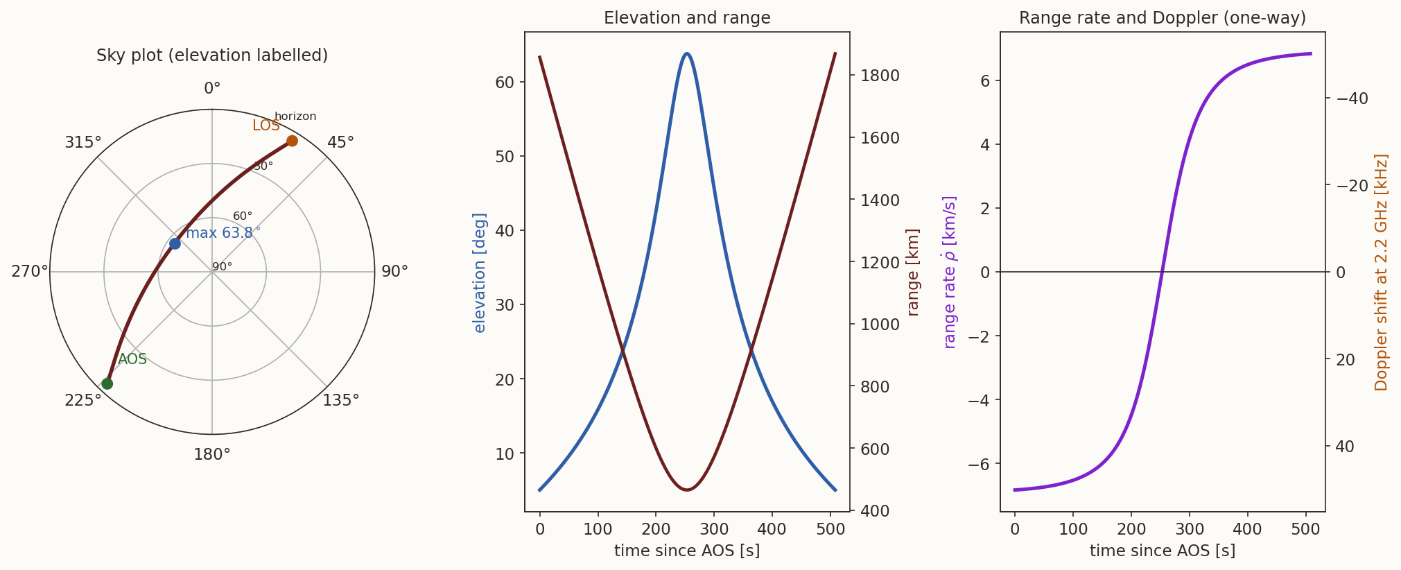
and in SEZ components \(\dot{\boldsymbol\rho}_{\rm SEZ}=\mathbf M\,\dot{\boldsymbol\rho}_{\rm ECEF}\). The second term is the velocity of the Earth-fixed point under the satellite, \(\omega_\oplus r\cos\varphi_{gc}\) (\(0.47\) km/s at the equator), and it is not small next to the satellite’s own \(7.7\) km/s: leaving it out changes \(\dot\rho\) by up to \(0.47\) km/s, comparable with the whole difference between the left and right ends of the range-rate curve of Figure 3.
Why not just differentiate \(\rho\) using the inertial velocity \(\mathbf v\)?
Answer
Because the station is not at rest in the inertial frame: it moves at \(\omega_\oplus\times\mathbf r_{\rm site}\). The range rate is the rate of change of the distance between the satellite and the station, and the station’s motion contributes. Equivalently, \(\dot\rho=\hat{\boldsymbol\rho}\cdot(\mathbf v-\mathbf v_{\rm site})\) in the inertial frame, and \(\mathbf v_{\rm site}=\boldsymbol\omega_\oplus\times\mathbf r_{\rm site}\); Equation 7 is the same statement written in the frame that rotates with the station.4.2 The three rates
The rate of the range is the component of the relative velocity along the line of sight. The azimuth and elevation rates follow from differentiating Equation 5. With \(\boldsymbol\rho_{\rm SEZ}=(\rho_S,\rho_E,\rho_Z)\) and \(\dot{\boldsymbol\rho}_{\rm SEZ}=(\dot\rho_S,\dot\rho_E,\dot\rho_Z)\),
\[ \boxed{\ \dot\rho=\frac{\boldsymbol\rho_{\rm SEZ}\cdot\dot{\boldsymbol\rho}_{\rm SEZ}}{\rho},\qquad \dot A=\frac{-\rho_S\,\dot\rho_E+\rho_E\,\dot\rho_S}{\rho_S^{2}+\rho_E^{2}},\qquad \dot\varepsilon=\frac{\dot\rho_Z-\dot\rho\,\sin\varepsilon}{\rho\cos\varepsilon}\ } \tag{8}\]
(for \(\dot A\), write \(A=\operatorname{atan2}(\rho_E,N)\) with \(N=-\rho_S\) and use \(\dot{(\arctan(E/N))}=(N\dot E-E\dot N)/(N^{2}+E^{2})\); for \(\dot\varepsilon\), differentiate \(\sin\varepsilon=\rho_Z/\rho\)). Note the singularities: the azimuth is undefined, and its rate unbounded, when the satellite passes through the zenith (\(\rho_S=\rho_E=0\)), and the elevation rate has \(\cos\varepsilon\) in the denominator for the same reason. A pass very close to overhead swings through all azimuths in a few seconds, which tracking antennas find hard to follow.
4.3 Doppler
A transmitter on the satellite sends a carrier of frequency \(\nu_t\). The receiver sees it shifted by
\[ \frac{\nu_r-\nu_t}{\nu_t}\approx-\frac{\dot\rho}{c} \tag{9}\]
to first order in \(\dot\rho/c\): approaching (\(\dot\rho<0\)) raises the frequency, receding lowers it. For a two-way link (the station transmits and a transponder returns the signal) the shift is twice as large, which is the \(-\tfrac12c\,\Delta\nu/\nu\) of the time note. A frequency is a clock measurement, so the clock error of the time note carries over: a fractional frequency error \(y\) in the reference is a range-rate error \(c\,y\).
4.4 A pass
Figure 3 shows the whole pass of the example orbit over the station, with a \(5^\circ\) elevation mask. The satellite rises (acquisition of signal, AOS) in the south-west at azimuth \(223.2^\circ\), reaches \(63.8^\circ\) in the north-west, and sets (loss of signal, LOS) in the north-east at \(31.4^\circ\), a total of \(507.9\) s later. At AOS and LOS it is \(1860\) km away and \(\dot\rho=\mp6.83\) km/s; at closest approach it is \(465\) km away and \(\dot\rho=0\), and the one-way Doppler shift of a \(2.2\) GHz carrier sweeps from \(+50.1\) kHz to \(-50.1\) kHz.
At the instant of the worked observation above, find the rates \(\dot A\), \(\dot\varepsilon\), \(\dot\rho\) and the one-way Doppler shift at \(2.2\) GHz.
What you should find
\(\dot A=0.1417^\circ\)/s, \(\dot\varepsilon=0.2494^\circ\)/s and \(\dot\rho=-6.008\) km/s (approaching), so the one-way shift is \(+44.09\) kHz. (The sign check: this is between AOS, where the shift is \(+50\) kHz, and closest approach, where it is zero.)5 From a radar observation to an orbit
A radar gives \((\rho,A,\varepsilon)\) and, with Doppler, their rates. That is six numbers at one instant, exactly what a state vector needs. The conversion is the forward chain run backwards.
- The line of sight in SEZ components, \(\boldsymbol\rho_{\rm SEZ}=\rho\hat{\mathbf u}\) from Equation 6, and its derivative \(\dot{\boldsymbol\rho}_{\rm SEZ}=\dot\rho\,\hat{\mathbf u}+\rho\,\dot{\hat{\mathbf u}}\), with \[ \dot{\hat{\mathbf u}}=\begin{bmatrix}\cos\varepsilon\sin A\,\dot A+\sin\varepsilon\cos A\,\dot\varepsilon\\ \cos\varepsilon\cos A\,\dot A-\sin\varepsilon\sin A\,\dot\varepsilon\\ \cos\varepsilon\,\dot\varepsilon\end{bmatrix}. \]
- Rotate to ECEF with \(\mathbf M^{\mathsf T}\) (the transpose is the inverse): \(\mathbf r_{\rm ECEF}=\mathbf r_{\rm site}+\mathbf M^{\mathsf T}\boldsymbol\rho_{\rm SEZ}\) and \(\dot{\boldsymbol\rho}_{\rm ECEF}=\mathbf M^{\mathsf T}\dot{\boldsymbol\rho}_{\rm SEZ}\).
- Rotate to the inertial frame, adding back the Earth’s rotation: \(\mathbf r=\mathbf R_3(\theta_G)\,\mathbf r_{\rm ECEF}\) and, inverting Equation 7, \(\mathbf v=\mathbf R_3(\theta_G)\bigl(\dot{\boldsymbol\rho}_{\rm ECEF}+\boldsymbol\omega_\oplus\times\mathbf r_{\rm ECEF}\bigr)\).
- Convert \((\mathbf r,\mathbf v)\) to orbital elements with the algorithm of the elements note.
Take the observation of the worked example, \((\rho,A,\varepsilon)=(868.822\ \text{km},\ 232.2122^\circ,\ 25.5051^\circ)\) with rates \((-6.0078\ \text{km/s},\ 0.141695^\circ/\text{s},\ 0.249444^\circ/\text{s})\) and \(\theta_G=100.727^\circ\). Rebuild the state vector and the elements.
What you should find
The chain returns \(\mathbf r=(-6668.678,\ 815.911,\ 1038.120)\) km and \(\mathbf v=(0.3193,\ -4.8834,\ 5.8893)\) km/s (to the digits of the input). The elements are \(a=6798.137\) km, \(e=0\) (to \(10^{-16}\): the orbit was built circular), \(i=51.64^\circ\) and \(\Omega=166.0^\circ\), with argument of latitude \(11.23^\circ\) (since \(n\,t=11.23^\circ\) after \(174.009\) s on the orbit’s own clock, and the argument of latitude was \(0\) at the epoch). With noise on the six measurements, of course, the elements would not be so tidy; Section 8 says how large the errors are.6 Angles only: right ascension and declination
An optical telescope, or a radar that cannot range, gives only the direction of the line of sight, two numbers. It is usually reported in the inertial sky coordinates: the topocentric right ascension \(\alpha\) and declination \(\delta\), which are the right ascension and declination of the direction from the site to the satellite. The direction cosines of the line of sight in the inertial frame are
\[ \hat{\boldsymbol\rho}=\bigl(\cos\delta\cos\alpha,\ \cos\delta\sin\alpha,\ \sin\delta\bigr)^{\mathsf T} =\mathbf R_3(\theta_G)\,\mathbf M^{\mathsf T}\hat{\mathbf u}, \tag{10}\]
where \(\hat{\mathbf u}\) is the unit line of sight in SEZ components of Equation 6. So, given \(A\) and \(\varepsilon\), we get \((\alpha,\delta)\) by the rotation, and vice versa. The same relation is the classical spherical-trigonometry triangle of positional astronomy (zenith, celestial pole, satellite). With the local sidereal time \(\Theta=\theta_G+\lambda\) (the right ascension of the meridian over the site) and the hour angle \(H=\Theta-\alpha\) (positive west of the meridian), it reads
\[ \boxed{\ \sin\delta=\sin\varphi\sin\varepsilon+\cos\varphi\cos\varepsilon\cos A,\qquad \cos\delta\,\sin H=-\cos\varepsilon\sin A,\qquad \cos\delta\,\cos H=\cos\varphi\sin\varepsilon-\sin\varphi\cos\varepsilon\cos A\ } \tag{11}\]
(here \(\varphi\) is the geodetic latitude, which is the astronomical latitude to the accuracy of a few arcseconds that we need). Given \((\delta,H)\) the same three equations, solved for \(\varepsilon\) and \(A\), give the horizon coordinates.
For the worked observation (\(A=232.2122^\circ\), \(\varepsilon=25.5051^\circ\), \(\varphi=12.97^\circ\), \(\lambda=77.59^\circ\), \(\theta_G=100.727^\circ\)), find \(\delta\) from Equation 11, the local sidereal time, and the topocentric \(\alpha\).
What you should find
\(\sin\delta=\sin12.97^\circ\sin25.505^\circ+\cos12.97^\circ\cos25.505^\circ\cos232.21^\circ=-0.4423\), so \(\delta=-26.25^\circ\). The local sidereal time is \(\Theta=100.727^\circ+77.59^\circ=178.317^\circ\) (\(11\) h \(53.3\) min). From the other two equations, \(H=52.68^\circ\), so \(\alpha=\Theta-H=125.64^\circ\). Rotating Equation 10 directly gives the same \((\alpha,\delta)=(125.64^\circ,-26.25^\circ)\).Three such directions at three times, with the observer’s position known, are enough in principle to determine an orbit. That is Gauss’s method of angles-only orbit determination, the most famous example of preliminary orbit determination, which the orbit-determination note will take up; it takes the direction cosines of Equation 10 and the site positions of Equation 2 as its data.
7 Is the satellite visible?
A station sees a satellite while its elevation is above the mask \(\varepsilon_{\min}\), a limit set by terrain, buildings, and atmospheric noise (typically \(5^\circ\) to \(10^\circ\)). For a circular orbit of radius \(r\) and a spherical Earth, the ground-tracks note gives the largest Earth central angle \(\psi_0\) between the station and the satellite’s sub-point at which the satellite is above the mask:
\[ \sin\eta=\frac{R_\oplus}{r}\cos\varepsilon_{\min},\qquad \psi_0=90^\circ-\varepsilon_{\min}-\eta, \]
where \(\eta\) is the nadir angle at which the station is seen from the satellite. If the satellite passes directly overhead and the Earth were not rotating, it crosses \(2\psi_0\) of its orbit above the mask, taking
\[ T_{\rm pass}\approx\frac{2\psi_0}{n},\qquad n=\sqrt{\mu/r^{3}} . \tag{12}\]
For the ISS orbit above a \(5^\circ\) mask, \(\eta=69.17^\circ\), \(\psi_0=15.83^\circ\) and \(T_{\rm pass}=490.5\) s, \(8.2\) min. The pass of Figure 3, \(63.8^\circ\) at its highest and not overhead, lasts \(507.9\) s: the Earth’s rotation, which carries the station along with the satellite, makes it a few percent longer. A satellite that reaches only \(20^\circ\) at its highest is above the mask for a much shorter part of its orbit, which is why pass durations in the tables of the ground-tracks note are averages over all passes.
Why does a higher orbit give a longer pass, though the satellite moves more slowly?
Answer
Both effects work in the same direction. A larger orbit radius \(r\) makes \(\eta\) smaller (the horizon is farther away, \(\sin\eta=R_\oplus\cos\varepsilon_{\min}/r\)), so \(\psi_0\) is larger: more of the orbit is in view. And it makes \(n\) smaller, so each radian takes longer. In Equation 12 both increase \(T_{\rm pass}\). At GEO the satellite never sets for the stations that see it at all.8 What limits the accuracy
Each measurement has an error, and the error in position at the satellite is the error of the observation times a lever arm.
- Angles. An angular error \(\delta\theta\) moves the apparent position of the satellite across the line of sight by \(\rho\,\delta\theta\). A pointing error of \(0.01^\circ\) at a range of \(1000\) km is \(175\) m. Refraction in the atmosphere bends the line of sight toward the zenith by an angle (Bennett’s empirical formula (Meeus 1998)) \[ R=\cot\!\Bigl(\varepsilon+\frac{7.31}{\varepsilon+4.4}\Bigr)\ \text{arcminutes}\qquad(\varepsilon\ \text{in degrees}), \] which is \(34.5'\) on the horizon, \(9.9'\) at \(\varepsilon=5^\circ\) and \(1.0'\) at \(\varepsilon=45^\circ\). A satellite at \(5^\circ\) is seen \(0.16^\circ\) too high, \(2.9\) km at \(1000\) km: this is why angle measurements below about \(10^\circ\) are avoided or corrected.
- The local vertical. Using the geocentric latitude in \(\mathbf M\) tilts the frame by up to \(0.192^\circ\), which is \(3.4\) km at \(1000\) km (Section 1.1).
- Range. A radar range is a time measurement, \(\rho=\tfrac12c\,\tau\), so its error is a clock error (the time note): \(10\) ns in \(\tau\) is \(1.5\) m. Range errors are along the line of sight and, for a radar, typically far smaller than the angle errors translated to metres, which is why a radar’s range is its best number.
- Range rate. A frequency error of \(0.1\) Hz on a \(2.2\) GHz carrier is \(13.6\) mm/s in \(\dot\rho\).
- Light time. The signal received at time \(t\) left the satellite at \(t-\rho/c\). At \(1860\) km that is \(6.2\) ms, during which the satellite moves \(48\) m. Precise orbit determination corrects for it, and the antenna’s pointing has to lead the line of sight by the same amount.
- Station position. The site vector of Equation 2 is known to centimetres with GPS and to a few metres from a map; a \(10\) m error in the station is a \(10\) m error in the satellite position.
In one paragraph. A station sits at geodetic latitude \(\varphi\) on the ellipsoid, at \(\mathbf r_{\rm site}\) of Equation 2. Its SEZ axes are the rows of \(\mathbf M\) (Equation 3). The satellite’s position is rotated into ECEF, subtracted from \(\mathbf r_{\rm site}\), and rotated by \(\mathbf M\) to give \(\boldsymbol\rho_{\rm SEZ}\) and, with Equation 5, the range, azimuth (from north, clockwise) and elevation. The rates use the velocity relative to the rotating Earth (Equation 7), and \(\dot\rho\) is what a Doppler measures. Run backwards, six radar numbers give a state vector and then the elements. An optical observation is the direction only, in right ascension and declination, which differ from the geocentric ones by parallax. The accuracy is set by the angle error times the range, the refraction, the local vertical, and the clock.
Summary
The numbers of this note are checked by topocentric-verify.py, using the helper module _topo.py; the figure scripts fig-topo-frames.py and fig-topo-pass.py draw the figures.
What we left out. (i) Precession, nutation and polar motion, which make the ECEF frame of this note an approximation at the metre level (the time note says so). (ii) Deflection of the vertical: the plumb line differs from the ellipsoid normal by up to tens of arcseconds because of local mass anomalies, so the “geodetic latitude” and the “astronomical latitude” are not quite equal. (iii) Aberration, the apparent shift of direction by \(v/c\) (about \(5''\) for a LEO satellite), and light-time, treated here only as a size. (iv) Atmospheric delay of ranging signals (ionosphere, troposphere), which adds metres to a range at low elevation.
Further reading. H. D. Curtis, Orbital Mechanics for Engineering Students, chapter 5 (topocentric coordinate systems, orbit determination from angle and range measurements); D. A. Vallado, Fundamentals of Astrodynamics and Applications (coordinate transformations, observation types, sensor models); the WGS 84 definition (National Imagery and Mapping Agency 2000); J. Meeus, Astronomical Algorithms (Meeus 1998), for refraction and the astronomical triangle.
Exercises
- The site vector. Compute \(\mathbf r_{\rm site}\) at the equator at the prime meridian, at sea level, and at the north pole. Check \(|\mathbf r_{\rm site}|=a\) and \(b\). (Answer: \((6378.137,0,0)\) km; \((0,0,6356.752)\) km.)
- Latitudes. Show that \(\tan\varphi_{gc}=(1-e^{2})\tan\varphi\) at \(h=0\), and find \(\varphi-\varphi_{gc}\) at \(\varphi=45^\circ\). (Answer: \(0.192^\circ\).)
- Matrix. Show that \(\mathbf M\) of Equation 3, with the rows reordered to \((\hat{\mathbf E},-\hat{\mathbf S},\hat{\mathbf Z})\), is the ENU matrix, and that its first row at \(\lambda=0\) is \((0,1,0)\).
- Overhead. A satellite is directly above the site at height \(h\). Find \(\boldsymbol\rho_{\rm SEZ}\), the range and the elevation. What is the azimuth? (Answer: \((0,0,h)\), \(h\), \(90^\circ\), and it is undefined.)
- Doppler rate. A \(2.2\) GHz transmitter on the ISS orbit passes at closest approach \(465\) km from a station. Treating the relative motion as a straight line at speed \(v\approx7\) km/s, show that \(\ddot\rho=v^{2}/\rho_{\min}\) at closest approach, and hence estimate the Doppler rate \(\dot\nu=-\nu\ddot\rho/c\) in Hz/s. (Answer: \(\ddot\rho\approx0.105\) km/s\(^2\) and \(\dot\nu\approx-770\) Hz/s; the exact value for the pass of Figure 3 is \(-800\) Hz/s.)
- Radar to state. Using the helper module, build the state from the observation of the worked example, and check that the elements come out as \(a=6798.137\) km, \(i=51.64^\circ\), \(\Omega=166.0^\circ\).
- Refraction. From Bennett’s formula, find the elevation at which refraction falls to one arcminute. (Answer: about \(45^\circ\).)
- Parallax. A satellite at \(r=7000\) km is seen at \(\varepsilon=10^\circ\) from a site on a spherical Earth of radius \(6378\) km. Find the angle between the topocentric and the geocentric directions of the satellite. (Hint: it is the angle at the satellite in the triangle formed with the site and the centre, and the sine rule gives it. Answer: \(\eta=\arcsin\bigl(\tfrac{6378}{7000}\cos10^\circ\bigr)=63.8^\circ\).)