Lambert’s Problem
Two positions, one time of flight — find the orbit, by \(p\)-iteration: existence, the algorithm, its limits, and the Lagrange coefficients
1 Where this note sits
Every orbit problem so far has been an initial-value problem: given \((\mathbf r,\mathbf v)\) now, find the state later, and Kepler’s equation did the work. This note turns the question around. Given two positions and the time between them, find the orbit. That is a boundary-value problem, and it is the basis of every targeted transfer, intercept and rendezvous in the chase deck.
The three are the same problem. Knowing the conic gives \(\mathbf v_1\) and \(\mathbf v_2\) by evaluating the velocity at the two points (Section 5). Knowing \(\mathbf v_1\) (or \(\mathbf v_2\)) gives a state vector, hence the orbit (the perifocal note), hence the other end.
We work in the orbital plane, with prograde motion. The transfer angle \(\Delta\theta\in(0,2\pi)\) is measured from \(\mathbf r_1\) to \(\mathbf r_2\) in the direction of motion: short way if \(\Delta\theta<\pi\), long way if \(\Delta\theta>\pi\). In three dimensions the plane is fixed by \(\mathbf r_1\) and \(\mathbf r_2\) (unless they are collinear with the focus), and the direction of motion then decides which of \(\Delta\theta\) and \(2\pi-\Delta\theta\) is the transfer angle.
Does a transfer exist? For any given \((\mathbf r_1,\mathbf r_2,\Delta t)\) the answer is the following, and the sections below prove it.
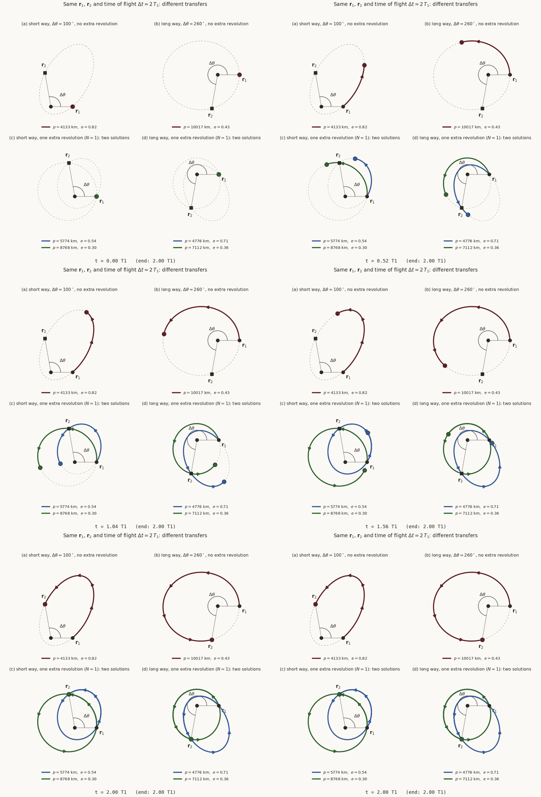
Figure 1 shows all four cases for one pair of points and one time of flight.
History. The problem is named after Johann Heinrich Lambert, who in Insigniores orbitae cometarum proprietates (1761) showed that the time on an elliptic arc depends only on the semi-major axis, the sum \(r_1+r_2\) and the chord \(c\), not on the eccentricity. Euler had proved the parabolic case about 1740, and Lambert reinvented it without knowing. Lagrange gave the first analytic expression for the time of flight in 1778. In 1801 Gauss used a method for this problem to find the orbit of the planet Ceres, which had been lost, from a \(3^\circ\) arc observed over 41 days; astronomers found it again where he had predicted. He set the method out in the Theoria motus (1809) (gauss1809?), which made it the central problem of orbit determination.
History: the modern solvers. The mid-1960s saw intensive work. Lancaster and Blanchard (1969) (lancaster1969?) reduced the problem to iterations that each need one inverse trigonometric or hyperbolic function; Battin and Vaughan (1984) (battinvaughan1984?) made it more robust; Gooding (1990) (gooding1990?) and Izzo (2015) (izzo2015?) followed. Richard Battin, at the MIT Instrumentation Laboratory, spent years on the problem for Apollo guidance (battin1964?). Today it is solved thousands of times per second in mission design: every point of a launch-window “porkchop” plot is one Lambert solution.
The plan, with every step done in full:
- The unknowns (Section 2). Two points and a focus leave a one-parameter family of conics; the time of flight selects one member.
- Labelling the family by \(p\) (Section 3). Given \(p\), the eccentricity and true anomaly follow in closed form. We find which \(p\) are allowed, and why.
- The clock (Section 4). Kepler’s equation for each conic type, the parabola, and the monotonicity that gives existence and uniqueness; then extra revolutions.
- Velocities (Section 5) and the \(p\)-iteration algorithm (Section 6), with two worked examples.
- Where \(p\)-iteration struggles (Section 7), which motivates universal variables.
- Velocities without elements (Section 8): the Lagrange coefficients.
| Symbol | Meaning |
|---|---|
| \(\mathbf r_1,\ \mathbf r_2\), \(r_1,\ r_2\) | the two position vectors and their lengths |
| \(\Delta\theta\), \(\Delta t\) | transfer angle (in the direction of motion) and time of flight |
| \(c=\lvert\mathbf r_2-\mathbf r_1\rvert\), \(s=\tfrac12(r_1+r_2+c)\) | chord and semi-perimeter |
| \(k=r_1r_2(1-\cos\Delta\theta)\), \(\ell=r_1+r_2\), \(m=r_1r_2(1+\cos\Delta\theta)\) | geometry constants used for the \(p\) window |
| \(p,\ e,\ a\) | semi-latus rectum, eccentricity, semi-major axis of the trial conic |
| \(f_1,\ f_2=f_1+\Delta\theta\) | true anomalies at the two points |
| \(A=p/r_1-1\), \(B=p/r_2-1\) | shorthand for \(e\cos f_1\) and \(e\cos f_2\) |
| \(N\) | number of complete revolutions added to the transfer |
| \(F,\,G,\,\dot F,\,\dot G\) | the Lagrange coefficients (written \(f,g,\dot f,\dot g\) in the universal-variables note) |
Throughout, \(\mu=398\,600.4418\ \mathrm{km^3/s^2}\) and \(R_\oplus=6378.137\) km.
2 The problem and its unknowns
2.1 Counting
Let the conic be
\[ r=\frac{p}{1+e\cos f}, \]
with the usual unknowns \(p\) and \(e\). A planar orbit is fixed by three elements \((p,e,\omega)\) plus one epoch. Put \(\mathbf r_1\) on the polar axis at angle \(\theta_1\), and let \(f_1\) be its true anomaly, so that the argument of periapsis is \(\omega=\theta_1-f_1\). The second point is at true anomaly \(f_2=f_1+\Delta\theta\). The orbit equation, written at the two points, gives
\[ r_1=\frac{p}{1+e\cos f_1}, \qquad r_2=\frac{p}{1+e\cos(f_1+\Delta\theta)} . \tag{1}\]
- Unknowns: \(p\), \(e\), \(f_1\).
- Equations: two.
So the geometry alone leaves one free parameter: a one-parameter family of conics through the two points (Figure 2). The time of flight is the third equation that pins down one member.
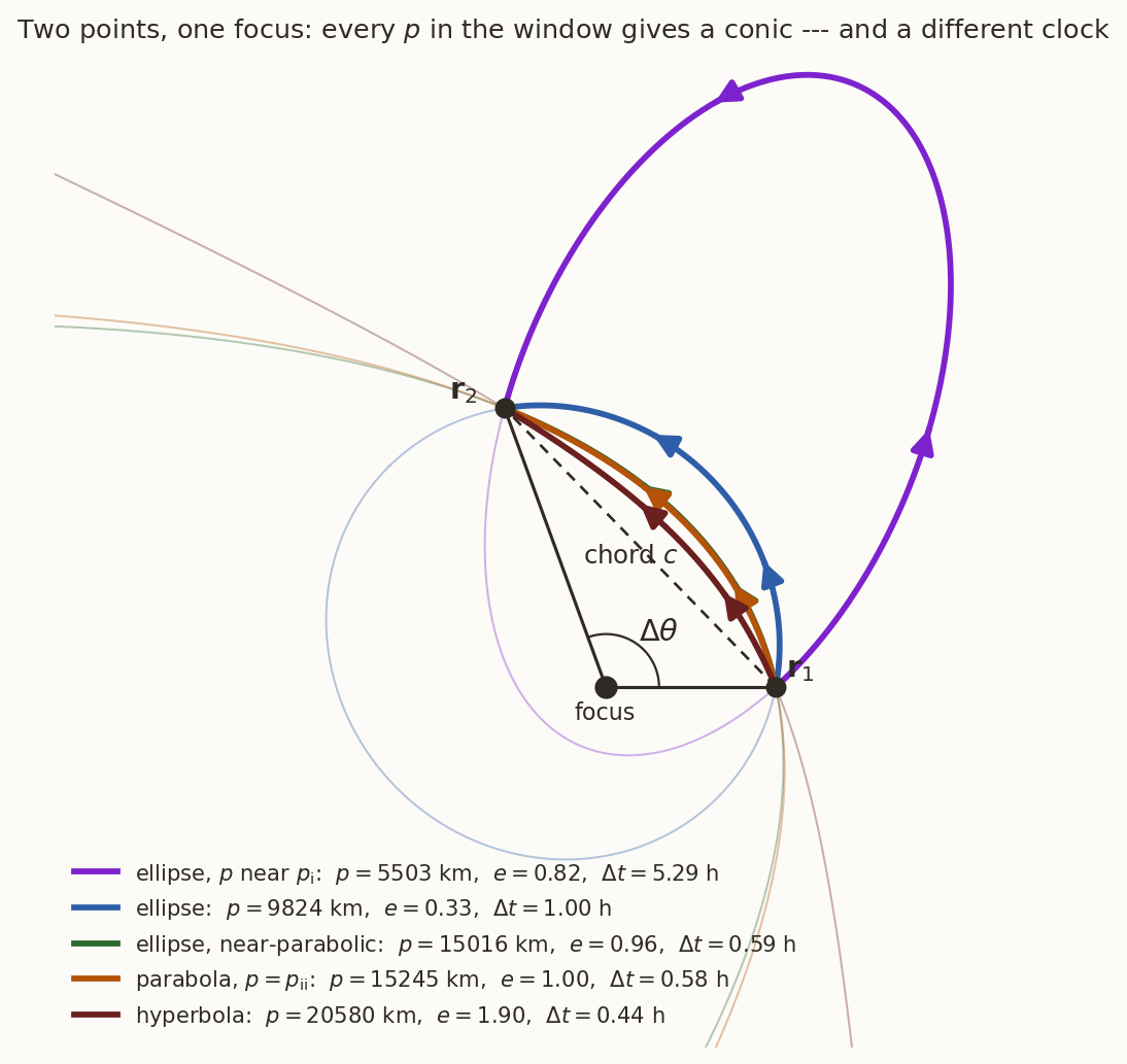
Why label by \(p\)? The semi-latus rectum \(p=h^{2}/\mu\) is finite for every conic (the semi-major axis \(a\) is not: it is infinite for the parabola and negative for the hyperbola), and it is a positive number that varies continuously across all three types. Given \(p\), the rest of the conic follows in closed form, as the next section shows.
3 Labelling the family by \(p\)
3.1 \(e\) and \(f_1\) in closed form
Write \(A=p/r_1-1\) and \(B=p/r_2-1\). Then Equation 1 says
\[ e\cos f_1=A, \qquad e\cos(f_1+\Delta\theta)=B . \]
Expand the second with the angle-addition formula, \(e\cos f_1\cos\Delta\theta-e\sin f_1\sin\Delta\theta=B\), and substitute the first, \(e\cos f_1=A\):
\[ \boxed{\ e\cos f_1=A, \qquad e\sin f_1=\frac{A\cos\Delta\theta-B}{\sin\Delta\theta}\ } \tag{2}\]
Given a trial \(p\), this delivers \(e=\sqrt{(e\cos f_1)^2+(e\sin f_1)^2}\) and \(f_1=\operatorname{atan2}(e\sin f_1,\,e\cos f_1)\) in closed form. Nothing is iterated yet. The same steps give the other end:
\[ e\cos f_2=B,\qquad e\sin f_2=e\sin f_1\cos\Delta\theta+e\cos f_1\sin\Delta\theta=\frac{A-B\cos\Delta\theta}{\sin\Delta\theta}, \tag{3}\]
since \(A\cos^{2}\Delta\theta-B\cos\Delta\theta+A\sin^{2}\Delta\theta=A-B\cos\Delta\theta\).
3.2 The eccentricity as a function of \(p\)
Square and add the two parts of Equation 2, and multiply by \(\sin^{2}\Delta\theta\):
\[ e^{2}\sin^{2}\Delta\theta=A^{2}+B^{2}-2AB\cos\Delta\theta . \tag{4}\]
This is a quadratic in \(p\). Substitute \(A=p/r_1-1\), \(B=p/r_2-1\) and expand:
\[ A^{2}+B^{2}-2AB\cos\Delta\theta =p^{2}\Big(\frac1{r_1^{2}}+\frac1{r_2^{2}}-\frac{2\cos\Delta\theta}{r_1r_2}\Big) -2p\Big(\frac1{r_1}+\frac1{r_2}\Big)\big(1-\cos\Delta\theta\big)+2\big(1-\cos\Delta\theta\big). \]
Multiply through by \(r_1^{2}r_2^{2}\). The bracket becomes \(c^{2}\) (the square of the chord, \(c^{2}=r_1^{2}+r_2^{2}-2r_1r_2\cos\Delta\theta\)), and the other coefficients become \(k\) and \(\ell\):
\[ r_1^{2}r_2^{2}\,e^{2}\sin^{2}\Delta\theta=c^{2}p^{2}-2k\ell\,p+2k\,r_1r_2 . \]
Now compute \(e^{2}-1\). Note \(r_1^{2}r_2^{2}\sin^{2}\Delta\theta=km\), because \(k\,m=r_1^{2}r_2^{2}(1-\cos^{2}\Delta\theta)\). So
\[ r_1^{2}r_2^{2}\sin^{2}\Delta\theta\,\big(e^{2}-1\big)=c^{2}p^{2}-2k\ell\,p+2k\,r_1r_2-km=c^{2}p^{2}-2k\ell\,p+k^{2}, \]
where the constant term collapses because \(2r_1r_2-m=r_1r_2(1-\cos\Delta\theta)=k\). The conic through the two points is parabolic (\(e=1\)) at the roots of
\[ c^{2}p^{2}-2k\ell\,p+k^{2}=0 . \]
Its roots are \(p=k\big(\ell\pm\sqrt{\ell^{2}-c^{2}}\big)/c^{2}\). Since \(\ell^{2}-c^{2}=2r_1r_2(1+\cos\Delta\theta)=2m\), we have \(c^{2}=\ell^{2}-2m=(\ell-\sqrt{2m})(\ell+\sqrt{2m})\), and so
\[ p_{\rm i}=\frac{k}{\ell+\sqrt{2m}}, \qquad p_{\rm ii}=\frac{k}{\ell-\sqrt{2m}} . \tag{5}\]
These are the two parabolas through the points. Since the quadratic has leading coefficient \(c^{2}\) and roots \(p_{\rm i}\), \(p_{\rm ii}\), it factorises, and we get the compact result
\[ \boxed{\ e^{2}=1+\frac{c^{2}\,(p-p_{\rm i})(p-p_{\rm ii})}{(r_1r_2\sin\Delta\theta)^{2}}\ } \tag{6}\]
Reading it off:
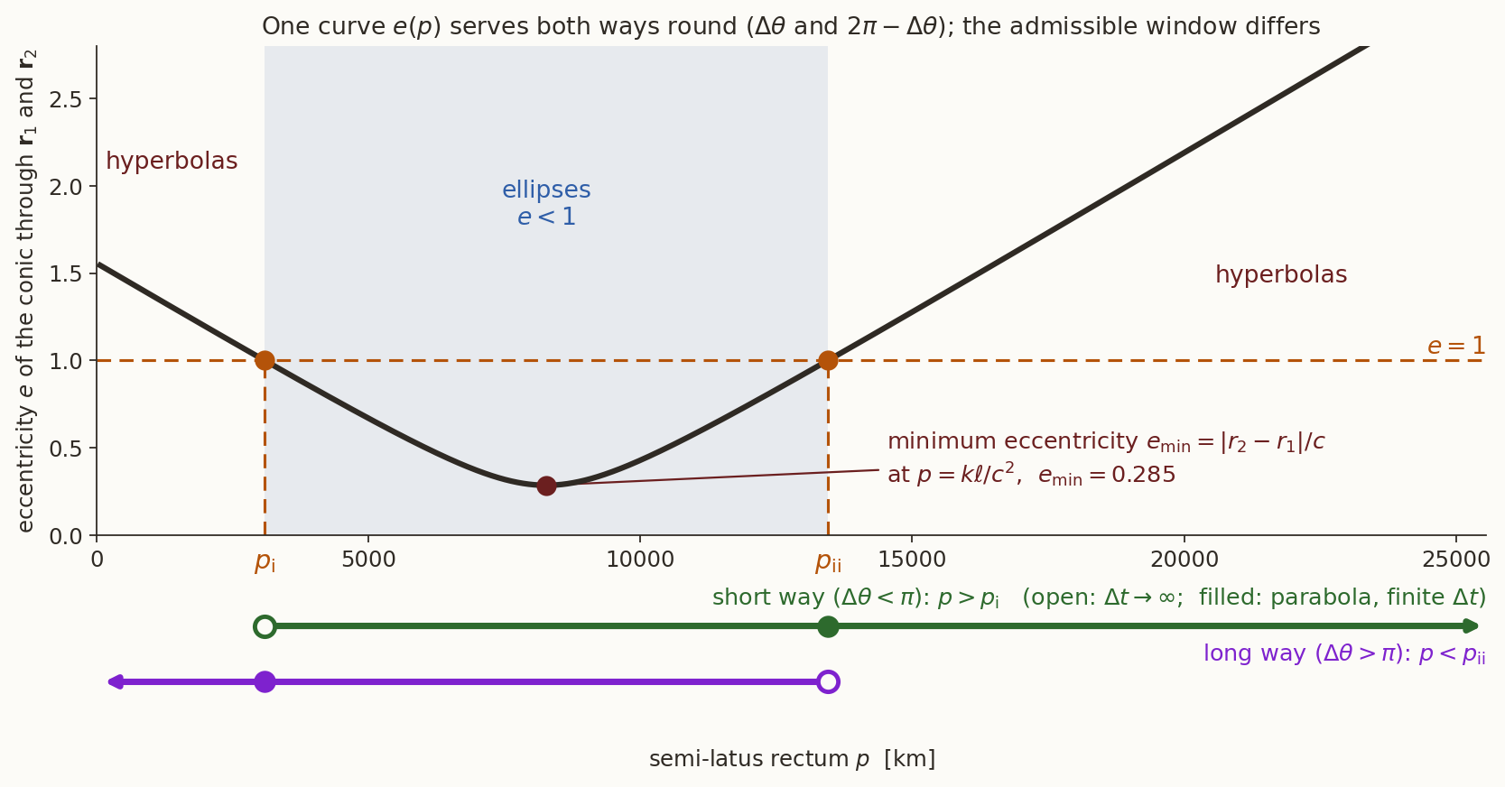
- Ellipse (\(e<1\)) for \(p_{\rm i}<p<p_{\rm ii}\); hyperbola (\(e>1\)) outside that interval. The type of the conic is known from \(p\) alone, with no iteration.
- \(e^{2}\) depends on \(\Delta\theta\) only through \(\cos\Delta\theta\) and \(\sin^{2}\Delta\theta\), so \(\Delta\theta\) and \(2\pi-\Delta\theta\) share the same \(e(p)\), \(p_{\rm i}\) and \(p_{\rm ii}\) (Figure 3). They differ only in which \(p\) are admissible.
- The minimum eccentricity. The quadratic is smallest at the midpoint of its roots, \(p_e=\tfrac12(p_{\rm i}+p_{\rm ii})=k\ell/c^{2}\). There \(p_{\rm ii}-p_{\rm i}=2k\sqrt{2m}/c^{2}\), so \(c^{2}(p_{\rm ii}-p_{\rm i})^{2}/4=2k^{2}m/c^{2}\); dividing by \(r_1^{2}r_2^{2}\sin^{2}\Delta\theta=km\), \[ e_{\min}^{2}=1-\frac{2k}{c^{2}}=\frac{c^{2}-2k}{c^{2}}=\frac{(r_2-r_1)^{2}}{c^{2}}, \qquad e_{\min}=\frac{\lvert r_2-r_1\rvert}{c}. \] No conic through the two points has a smaller eccentricity. (For \(r_1=r_2\) the minimum is the circle, as it should be.)
3.3 Which values of \(p\) are allowed?
Equation 2 returns a real \(e\) and an angle \(f_1\) for every \(p>0\), so a conic of parameter \(p\) through both points always exists. But we need an arc of it, run in the direction of motion from \(\mathbf r_1\) to \(\mathbf r_2\), that sweeps the true anomaly \(\Delta\theta\). Call \(p\) admissible if there is one.
- Ellipse (\(e<1\)): every true anomaly occurs, so the arc from \(f_1\) to \(f_1+\Delta\theta\) exists. Always admissible.
- Parabola or hyperbola (\(e\ge1\)): the true anomaly is confined to \(\lvert f\rvert<f_\infty=\cos^{-1}(-1/e)\) (with \(f_\infty=\pi\) for the parabola). Admissible if and only if both \(f_1\) and \(f_2=f_1+\Delta\theta\) lie in this interval (with \(f_1\) taken from \(\operatorname{atan2}\), in \((-\pi,\pi]\)). Otherwise the arc would have to cross an asymptote.
Where can admissibility change? On the hyperbolic range (\(e>1\)) neither \(f_1\) nor \(f_2\) can ever reach \(\pm f_\infty\) for a finite \(p\): that would need \(1+e\cos f_k=0\), but \(1+e\cos f_k=p/r_k>0\). So within each connected hyperbolic interval of \(p\) (that is, \(p<p_{\rm i}\) and \(p>p_{\rm ii}\)) the admissibility is constant, and one test value settles each interval.
- \(p\to\infty\). \(e\to\infty\) and \(f_\infty\to\pi/2\): the hyperbola degenerates into a straight line run infinitely fast. A straight line joins \(\mathbf r_1\) to \(\mathbf r_2\) along the chord, sweeping an angle \(<\pi\) as seen from the focus. So \(p>p_{\rm ii}\) is admissible for the short way and not for the long way.
- \(p\to0\). Then \(A=B=-1\), and Equation 4 gives \(e^{2}\sin^{2}\Delta\theta=2(1-\cos\Delta\theta)\), that is \(e=1/\lvert\cos(\Delta\theta/2)\rvert\). Both points have \(1+e\cos f_k=p/r_k\to0\), so they sit near the two asymptotes, \(f_1\approx-f_\infty\) and \(f_2\approx+f_\infty\), and the arc between them sweeps \(2f_\infty=2\cos^{-1}\!\big(-\lvert\cos\tfrac{\Delta\theta}{2}\rvert\big)\). For \(\Delta\theta>\pi\) this is \(\Delta\theta\) (since \(\cos(\Delta\theta/2)<0\) there), exactly what we need. For \(\Delta\theta<\pi\) it is \(2\pi-\Delta\theta\neq\Delta\theta\). So \(p<p_{\rm i}\) is admissible for the long way and not for the short way.
| admissible \(p\) | ellipse | hyperbola | |
|---|---|---|---|
| short way, \(\Delta\theta<\pi\) | \(p_{\rm i}<p<\infty\) | \(p_{\rm i}<p<p_{\rm ii}\) | \(p>p_{\rm ii}\) |
| long way, \(\Delta\theta>\pi\) | \(0<p<p_{\rm ii}\) | \(p_{\rm i}<p<p_{\rm ii}\) | \(p<p_{\rm i}\) |
The parabolas. Exactly one of the two parabolas is admissible for each way, and it is the one that joins the hyperbolic and elliptic ranges inside the window: \(p_{\rm ii}\) for the short way, \(p_{\rm i}\) for the long way. The other one is only approached from the elliptic side, by ellipses whose arc runs round a very distant apoapsis, so the time of flight diverges there (\(\Delta t\to\infty\) as \(p\to p_{\rm i}\) for the short way, and as \(p\to p_{\rm ii}\) for the long way). For the admissible parabola the unwrapped \(f_2\) stays below \(\pi\) and the time is finite; it is computed in Section 4.3.
(codes/lambert-verify.py checks Table 2 against the direct test, with the unwrapped anomalies, on \(15\,440\) random cases.)
4 The clock
With \((p,e,f_1,f_2)\) known, the time of flight is Kepler’s equation, twice, with a different form for each conic.
4.1 Ellipse (\(e<1\))
Write the same radius in two ways, \(r=a(1-e\cos E)=p/(1+e\cos f)\), with \(p=a(1-e^{2})\). Then \(1-e\cos E=(1-e^{2})/(1+e\cos f)\), so \(e\cos E=(e\cos f+e^{2})/(1+e\cos f)\) and
\[ \cos E=\frac{e+\cos f}{1+e\cos f}. \]
The half-angle relation follows from \(\tan^{2}(E/2)=(1-\cos E)/(1+\cos E)\):
\[ \tan^{2}\frac E2=\frac{(1+e\cos f)-(e+\cos f)}{(1+e\cos f)+(e+\cos f)} =\frac{(1-e)(1-\cos f)}{(1+e)(1+\cos f)}=\frac{1-e}{1+e}\tan^{2}\frac f2 . \]
\(E\) and \(f\) lie in the same half-plane (both grow together from periapsis), so \(\tan\frac E2=\sqrt{(1-e)/(1+e)}\,\tan\frac f2\). For computation use the form that is safe at \(f=\pi\) and for every \(f\), \(E=2\operatorname{atan2}\!\big(\sqrt{1-e}\,\sin\tfrac f2,\ \sqrt{1+e}\,\cos\tfrac f2\big)\). Kepler’s equation \(M=E-e\sin E\) and \(M=n\,(t-t_p)\) with \(n=\sqrt{\mu/a^{3}}\) give
\[ \begin{aligned} \Delta t&=\frac{\Delta E-e\,\big[\sin(E_1+\Delta E)-\sin E_1\big]}{n},\\ \Delta E&=\big[(E_2-E_1)\bmod2\pi\big]+2\pi N . \end{aligned} \tag{7}\]
For \(N=0\) take \(E_2-E_1\in(0,2\pi)\), no complete revolution. Each extra revolution adds \(2\pi\) to \(\Delta E\), and since sines are periodic that adds exactly one period \(T=2\pi/n\) to the time: \(\Delta t_N=\Delta t_0+N\,T(p)\).
4.2 Hyperbola (\(e>1\))
The same steps with \(a=p/(1-e^{2})<0\) and \(r=\lvert a\rvert(e\cosh H-1)=p/(1+e\cos f)\) give \(\cosh H=(e+\cos f)/(1+e\cos f)\) and
\[ \tanh^{2}\frac H2=\frac{\cosh H-1}{\cosh H+1}=\frac{e-1}{e+1}\tan^{2}\frac f2 . \]
With the hyperbolic Kepler equation \(M_h=e\sinh H-H\) and \(n_h=\sqrt{\mu/(-a)^{3}}\):
\[ \begin{aligned} \tanh\frac H2&=\sqrt{\frac{e-1}{e+1}}\tan\frac f2,\qquad M_h=e\sinh H-H,\\ \Delta t&=\frac{M_{h,2}-M_{h,1}}{n_h}. \end{aligned} \tag{8}\]
Both anomalies must satisfy \(\lvert f\rvert<f_\infty\), as in Section 3.3. There are no complete revolutions: \(N=0\).
4.3 Parabola (\(e=1\))
For \(e=1\), \(a\) is infinite and neither form applies. Integrate the angular-momentum equation \(dt=r^{2}\,df/h\) directly, with \(r=p/(1+\cos f)=\tfrac p2\sec^{2}\tfrac f2\) and \(h=\sqrt{\mu p}\). With \(D=\tan\tfrac f2\), \(df=2\,dD/(1+D^{2})\) and \(\sec^{2}\tfrac f2=1+D^{2}\):
\[ r^{2}\,df=\frac{p^{2}}{4}(1+D^{2})^{2}\,\frac{2\,dD}{1+D^{2}}=\frac{p^{2}}{2}(1+D^{2})\,dD, \]
and integrating, with \(p^{2}/\sqrt{\mu p}=\sqrt{p^{3}/\mu}\) (Barker’s equation):
\[ \Delta t=\frac12\sqrt{\frac{p^{3}}{\mu}}\Big[\Big(D_2+\frac{D_2^{3}}{3}\Big)-\Big(D_1+\frac{D_1^{3}}{3}\Big)\Big], \qquad D_k=\tan\frac{f_k}{2}. \]
For the parabola through the two points the same time has a closed form in the geometry alone, Euler’s parabolic theorem:
\[ \Delta t_{\rm par}=\frac13\sqrt{\frac2\mu}\Big[s^{3/2}\mp(s-c)^{3/2}\Big], \tag{9}\]
with the minus sign for the short way and the plus sign for the long way. (codes/lambert-verify.py checks that Equation 9 equals Barker’s equation at the admissible parabola, for six geometries and both ways.) This is the threshold of the existence result in Section 1: a given \(\Delta t\) is an ellipse for \(\Delta t>\Delta t_{\rm par}\) and a hyperbola for \(\Delta t<\Delta t_{\rm par}\). For Example 1 below, \(\Delta t_{\rm par}=2.238\) h.
Lambert’s theorem, in Lagrange’s form. For an elliptic arc, \(n\,\Delta t=(\alpha-\sin\alpha)-(\beta-\sin\beta)\), where \(\sin^{2}(\alpha/2)=s/2a\) and \(\sin^{2}(\beta/2)=(s-c)/2a\). The right-hand side contains only \(a\), \(s\) and \(c\): the time depends on the eccentricity not at all. (The standard branch rules apply: \(\beta\to-\beta\) for the long way, and \(\alpha\to2\pi-\alpha\) if the arc contains apoapsis.) For Example 1, with \(c=48\,820.2\) km and \(s=48\,831.2\) km, \(\alpha=2.64678\), \(\beta=0.02907\) and the formula returns \(14\,400.0\) s.
4.4 The clock is monotone in \(p\)
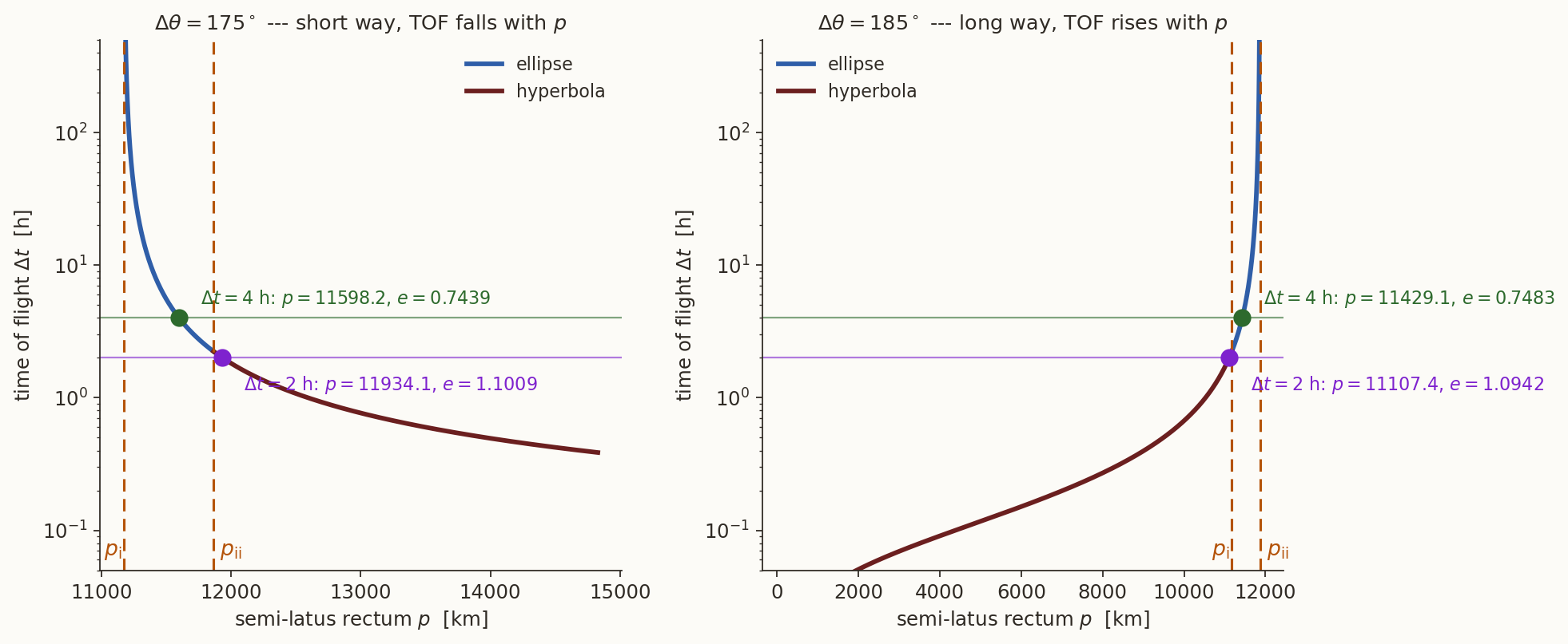
Put the pieces together: for a given \(\Delta\theta\) and a trial \(p\) in the admissible window, Equation 2 gives \((e,f_1)\) and the matching clock gives \(\Delta t(p)\). For zero revolutions this is a monotone function of \(p\) across the whole window (Figure 4):
- Short way: \(\Delta t\) falls as \(p\) grows, from \(+\infty\) at \(p\to p_{\rm i}^{+}\) (ellipses running round a distant apoapsis), through the parabolic value \(\Delta t_{\rm par}\) at \(p_{\rm ii}\), down to \(0\) as \(p\to\infty\) (numerically \(\Delta t\propto p^{-1/2}\) there).
- Long way: \(\Delta t\) rises as \(p\) grows, from \(0\) at \(p\to0\) (a fast dive past the focus), through \(\Delta t_{\rm par}\) at \(p_{\rm i}\), up to \(+\infty\) as \(p\to p_{\rm ii}^{-}\).
So each \(\Delta t\in(0,\infty)\) is reached exactly once: this is the existence and uniqueness statement of Section 1. We have not proved the monotonicity analytically; codes/lambert-verify.py confirms it on a scan of \(116\) random geometries (both ways, over the whole window, ellipse and hyperbola), and checks both limits.
4.5 More than one revolution
Allow \(N\) complete revolutions. Only ellipses can complete a revolution, so \(N\ge1\) lives entirely in \(p_{\rm i}<p<p_{\rm ii}\), and by Equation 7
\[ \Delta t_N(p)=\Delta t_0(p)+N\,T(p),\qquad T(p)=2\pi\sqrt{\frac{a^{3}}{\mu}},\ \ a=\frac{p}{1-e^{2}} . \]
At both ends of the window the period diverges (\(e\to1\) gives \(a\to\infty\)), so \(\Delta t_N\to\infty\) at both ends, and a continuous function that is infinite at both ends has a minimum \(\Delta t_{\min}(N)\) in between. The clock is therefore no longer monotone: for \(\Delta t\) below the minimum there is no solution, and above it there are two, one on each side of the minimum. Bisection alone can no longer be trusted: it must be told which side to search.
For the geometry of Figure 1 (\(r_2/r_1=11/7\)), the minimum times are
| \(N=0\) | \(N=1\) | \(N=2\) | |
|---|---|---|---|
| short way, \(\Delta\theta=100^\circ\) | \(0.248\,T_1\) | \(1.766\,T_1\) | \(3.013\,T_1\) |
| long way, \(\Delta\theta=260^\circ\) | \(0.271\,T_1\) | \(1.790\,T_1\) | \(3.037\,T_1\) |
At \(\Delta t=2T_1\) both \(N=0\) and \(N=1\) exist (one and two solutions per way, as in Figure 1) and \(N=2\) does not, since \(2T_1<3.013\,T_1\). In Figure 1 (c) both \(N=1\) orbits sweep \(100^\circ+360^\circ=460^\circ\) of true anomaly in the same time; the green one (\(e=0.30\)) is nearly circular, the blue one (\(e=0.54\)) a more eccentric ellipse that dives closer to the focus and is flown faster there.
5 Velocities
Once \(p\) is found, angular momentum \(h=\sqrt{\mu p}\) and the orbit equation give the radial and transverse speeds at any true anomaly. (This is the result of the perifocal note, derived there in full; here is the short version.) From \(h=r^{2}\dot f\), \(v_\theta=r\dot f=h/r\). Differentiating \(r=p/(1+e\cos f)\) in time, \(\dot r=\dfrac{p\,e\sin f}{(1+e\cos f)^{2}}\,\dot f=\dfrac{r^{2}\dot f}{p}\,e\sin f=\dfrac hp\,e\sin f\). So
\[ v_\theta=\frac{h}{r}=\sqrt{\frac{\mu}{p}}\,(1+e\cos f), \qquad v_r=\dot r=\sqrt{\frac{\mu}{p}}\,e\sin f . \tag{10}\]
At the two ends, \(1+e\cos f_k=p/r_k\), and Equation 2 and Equation 3 give \(e\sin f_k\), so the velocities need neither \(e\) nor \(f\) separately:
\[ \begin{aligned} v_{r1}&=\sqrt{\frac{\mu}{p}}\;\frac{A\cos\Delta\theta-B}{\sin\Delta\theta},&\qquad v_{\theta1}&=\frac{\sqrt{\mu p}}{r_1},\\[2pt] v_{r2}&=\sqrt{\frac{\mu}{p}}\;\frac{A-B\cos\Delta\theta}{\sin\Delta\theta},&\qquad v_{\theta2}&=\frac{\sqrt{\mu p}}{r_2}. \end{aligned} \tag{11}\]
Rotate into the inertial frame with the unit vectors at each end, \(\hat{\mathbf u}_r(\theta)=(\cos\theta,\sin\theta)\) and \(\hat{\mathbf u}_\theta(\theta)=(-\sin\theta,\cos\theta)\):
\[ \mathbf v_k=v_{r,k}\,\hat{\mathbf u}_r(\theta_k)+v_{\theta,k}\,\hat{\mathbf u}_\theta(\theta_k), \qquad k=1,2 . \]
6 The \(p\)-iteration algorithm
- The secant update is \(p_{k+1}=p_k-\big(\Delta t_k-\Delta t\big)\dfrac{p_k-p_{k-1}}{\Delta t_k-\Delta t_{k-1}}\). It converges superlinearly (order \(\approx1.62\)), where bisection only gains one binary digit per step.
- If a secant step leaves the window, fall back to bisection on the current bracket. A bracket always exists for \(N=0\) (Section 4.4): \((p_{\rm i},p_{\rm ii})\) if an ellipse is expected, with the long way the mirror image.
- Bisection from the window of Example 1 below (\(690\) km wide) down to \(10^{-6}\) km takes about \(30\) steps; the secant method takes seven updates.
6.1 Example 1 — LEO \(\to\) GEO in four hours
Given \(r_1=6678.137\) km, \(r_2=42\,164\) km, \(\Delta\theta=175^\circ\), \(\Delta t=4\) h \(=14\,400\) s. Here \(\cos175^\circ=-0.996195\) and \(1-\cos\Delta\theta=1.996195\).
Window. With \(k=5.62082\times10^{8}\) km\(^{2}\), \(\ell=48\,842.137\) km and \(m=1.07149\times10^{6}\) km\(^{2}\),
\[ p_{\rm i}=11\,173.263\ \mathrm{km}, \qquad p_{\rm ii}=11\,863.724\ \mathrm{km}. \]
The parabola at \(p_{\rm ii}\) takes \(2.238\) h \(<4\) h (Euler’s theorem, Equation 9, gives the same), so the answer is an ellipse. Secant iteration from \(p=11\,300\) and \(11\,800\) km converges in seven updates; every iterate stays inside the window:
| step | \(p\) [km] | \(\Delta t\) [h] | \(e\) |
|---|---|---|---|
| 0 | \(11300\) | \(19.207\) | \(0.847\) |
| 1 | \(11800\) | \(2.507\) | \(0.918\) |
| 2 | \(11755.29\) | \(2.736\) | \(0.866\) |
| 3 | \(11508.72\) | \(5.364\) | \(0.727\) |
| 4 | \(11636.70\) | \(3.598\) | \(0.764\) |
| 5 | \(11607.55\) | \(3.894\) | \(0.748\) |
| 6 | \(11597.17\) | \(4.012\) | \(0.7435\) |
| 7 | \(11598.19\) | \(3.9997\) | \(0.7440\) |
| 8 | \(\mathbf{11598.16}\) | \(\mathbf{4.0000}\) | \(\mathbf{0.74395}\) |
The converged arc. \(p=11\,598.163\) km gives, from Equation 2,
\[ A=0.736736,\quad B=-0.724927,\quad e\sin f_1=-0.103326, \]
\[ e=0.74395,\qquad f_1=-7.984^\circ,\qquad f_2=167.016^\circ . \]
Clock check. \(a=25\,973.20\) km, \(n=1.508276\times10^{-4}\) rad/s, \(E_1=-0.053465\), \(E_2=2.564252\), so \(M_1=-0.013709\), \(M_2=2.158208\) and
\[ \frac{M_2-M_1}{n}=\frac{2.171917}{1.508276\times10^{-4}}=14\,400.0\ \mathrm{s}\ \checkmark \]
Velocities from Equation 10, \((v_r,\,v_\theta)\) in km/s:
\[ \mathbf v_1=(-0.60573,\ 10.18142), \qquad \mathbf v_2=(0.97986,\ 1.61258), \]
with flight-path angles \(-3.40^\circ\) at departure and \(31.28^\circ\) at arrival. Departing from the circular LEO speed \(7.7258\) km/s and arriving into the circular GEO speed \(3.0747\) km/s:
\[ \boxed{\begin{aligned} &\Delta v_1=2.52926,\quad \Delta v_2=1.76006,\quad \Delta v_{\rm total}=4.28932\ \mathrm{km/s}\\ &\text{Hohmann: } 3.89255\ \mathrm{km/s}\text{ in } 5.275\ \mathrm h \end{aligned}} \]
Saving \(1.3\) hours of the Hohmann time of flight costs \(0.40\) km/s.
6.2 Example 2 — the same trip in two hours
Now \(\Delta t=2\) h \(<2.238\) h, so the answer must be a hyperbola, \(p>p_{\rm ii}\). Secant from \(p=11\,900\) and \(12\,200\) km:
| \(p\) [km] | \(\Delta t\) [h] | \(e\) |
|---|---|---|
| \(11900\) | \(2.1088\) | \(1.051\) |
| \(12200\) | \(1.4243\) | \(1.538\) |
| \(11947.69\) | \(1.9597\) | \(1.121\) |
| \(11928.68\) | \(2.0166\) | \(1.093\) |
| \(11934.21\) | \(1.9997\) | \(1.101\) |
| \(\mathbf{11934.10}\) | \(\mathbf{2.0000}\) | \(\mathbf{1.10087}\) |
The converged hyperbola has \(f_1=-44.363^\circ\) and \(f_2=130.637^\circ\), both inside \(f_\infty=155.281^\circ\). \(H_1=-0.179153\), \(H_2=1.037685\), so \(M_{h,1}=-0.019128\), \(M_{h,2}=0.321009\). With \(a=-56\,316.04\) km and \(n_h=4.724118\times10^{-5}\ \mathrm{s^{-1}}\):
\[ \frac{M_{h,2}-M_{h,1}}{n_h}=\frac{0.340137}{4.724118\times10^{-5}}=7200\ \mathrm s\ \checkmark \]
The velocities are \(\mathbf v_1=(-4.44847,\ 10.32782)\) and \(\mathbf v_2=(4.82797,\ 1.63577)\) km/s, and
\[ \boxed{\ \Delta v_1=5.15360,\quad \Delta v_2=5.03783,\quad \Delta v_{\rm total}=10.19143\ \mathrm{km/s}\ } \]
Saving the last \(14\) minutes over the parabola (\(2.238\) h \(\to2\) h) more than doubles the bill.
(codes/lambert-verify.py reproduces both iteration tables and every number above.)
7 Where \(p\)-iteration struggles
7.1 Difficulty 1: three clocks for three conics
The time equation is different for \(e<1\), \(e=1\) and \(e>1\), and we do not know which applies until \(p\) is known.
- Starting guesses on one side of \(p_{\rm ii}\) may converge to the other, so the code must switch formulas mid-iteration.
- Near \(e=1\) each formula is a ratio of vanishing quantities: \(a\to\infty\), \(n\to0\), \(\Delta M\to0\).
Where the digits go. Look at the elliptic clock when \(e\to1\) at fixed \(p\). Then \(a=p/(1-e^{2})\to\infty\), and the anomalies shrink, \(E\sim\sqrt{(1-e)/(1+e)}\;2\tan\tfrac f2\to0\). The mean anomaly \(M=E-e\sin E\) is a difference of two nearly equal numbers:
\[ M=(1-e)\,E+e\,(E-\sin E)\approx(1-e)\,E+\frac{E^{3}}{6}, \]
which is of order \((1-e)^{3/2}\) while each of \(E\) and \(e\sin E\) is of order \((1-e)^{1/2}\). So a relative cancellation of order \(1-e\): the relative error of \(\Delta t\) in double precision grows like \(\varepsilon_{\rm mach}/(1-e)\). Measured against 50-digit arithmetic, just below \(p_{\rm ii}\) in the geometry of Example 1:
| \(1-e\) | \(1.6\times10^{-5}\) | \(1.6\times10^{-8}\) | \(1.6\times10^{-11}\) | \(1.6\times10^{-13}\) |
|---|---|---|---|---|
| relative error in \(\Delta t\) | \(2.2\times10^{-12}\) | \(1.6\times10^{-9}\) | \(2.8\times10^{-6}\) | \(3.0\times10^{-4}\) |
Digits leak away exactly where the physics is perfectly smooth: nothing special happens to the trajectory at \(e=1\) (Equation 9 is smooth across it).
7.2 Difficulty 2: the window moves
The admissible interval \((p_{\rm i},\infty)\) or \((0,p_{\rm ii})\) depends on \(r_1\), \(r_2\) and \(\Delta\theta\). A trial \(p\) outside it gives a conic that does not join the two points in the direction of motion (a hyperbolic arc would have to cross its asymptote). The algorithm must compute the bracket before it can take a single step.
7.3 Difficulty 3: the window pinches at \(180^\circ\)
At \(\Delta\theta=\pi\), Equation 1 gives \(e\cos f_1=A\) and \(-e\cos f_1=B\), so \(A+B=0\):
\[ \frac{p}{r_1}+\frac{p}{r_2}=2 \quad\Longrightarrow\quad \boxed{\ p=p_H\equiv\frac{2r_1r_2}{r_1+r_2}\ } \]
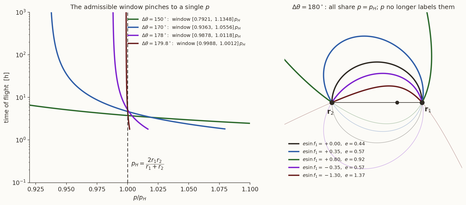
the harmonic mean of the two radii: the \(p\) of the Hohmann ellipse, and of every other conic whose chord passes through the focus. The free parameter becomes \(e\sin f_1\), and \(p\) can no longer label the family (Figure 5, right).
How fast does the window close? Near \(\pi\), \(k\to2r_1r_2\), \(c\to\ell\) and \(\sqrt{2m}=2\sqrt{r_1r_2}\,\lvert\cos\tfrac{\Delta\theta}{2}\rvert\approx\sqrt{r_1r_2}\,(\pi-\Delta\theta)\), so from Equation 5
\[ p_{\rm ii}-p_{\rm i}=\frac{2k\sqrt{2m}}{c^{2}}\approx\frac{4\,(r_1r_2)^{3/2}}{(r_1+r_2)^{2}}\,(\pi-\Delta\theta): \]
linear in the distance from \(180^\circ\). For the radii of Example 1 and \(\Delta\theta=179.9^\circ\) the window is \(13.83\) km wide around \(p_H=11\,530.08\) km (the formula gives \(13.83\)), and the clock is almost vertical across it: \(\Delta t=5\) h needs \(p=11\,530.375\) km and \(\Delta t=1.8\) h needs \(p=11\,539.775\) km, a change of only \(9.4\) km (Figure 5, left, shows the same effect at \(179.8^\circ\) and below).
7.4 Difficulty 4: more than one revolution
As shown in Section 4.5, the clock for \(N\ge1\) is not monotone: it has a minimum, and each \(\Delta t\) above it has two solutions. Bisection alone can no longer be trusted.
7.5 What we would like instead
Difficulties 1 and 2 are artefacts of the variable, not of the physics. We want:
- one iteration variable, defined for every conic;
- one time-of-flight equation, smooth straight through \(e=1\);
- an iteration range that does not have to be computed from the geometry first.
That is exactly what the universal-variable formulation provides: a single anomaly-like variable whose sign tells you the conic, and a single Kepler-like equation that reduces to the elliptic, parabolic and hyperbolic forms as special cases. It is the subject of the universal-variables note.
8 Velocities without elements: the Lagrange coefficients
8.1 The idea: stay in the plane of \(\mathbf r_1\) and \(\mathbf v_1\)
Section 5 found \(\mathbf v_1\) by first computing \(e\) and \(f_1\) (Equation 11 already hides them). We can skip that detour. The motion is planar, and \(\mathbf r_1\), \(\mathbf v_1\) are not parallel (unless the orbit is a straight line through the focus). So they form a basis for the orbital plane, and every later position and velocity is a combination of them:
\[ \boxed{\ \mathbf r_2=F\,\mathbf r_1+G\,\mathbf v_1, \qquad \mathbf v_2=\dot F\,\mathbf r_1+\dot G\,\mathbf v_1\ } \tag{12}\]
- \(F\), \(G\), \(\dot F\), \(\dot G\) are scalars: the Lagrange coefficients.
- The second equation is the time derivative of the first (\(\mathbf r_1\), \(\mathbf v_1\) are fixed vectors; only the coefficients change as the end point moves), hence the dots.
- Units: \(F\) and \(\dot G\) are dimensionless, \(G\) is a time, \(\dot F\) is an inverse time.
The payoff. Once \(F\) and \(G\) are known, the first equation solves for the unknown velocity: \(\mathbf v_1=(\mathbf r_2-F\,\mathbf r_1)/G\).
The goal. Express \(F\), \(G\), \(\dot G\) using only \(r_1\), \(r_2\), \(\Delta\theta\) and \(p\).
8.2 Step 1: components in the frame at departure
Use the radial and transverse unit vectors at \(\mathbf r_1\): \(\hat{\mathbf u}_r\) along \(\mathbf r_1\), and \(\hat{\mathbf u}_\theta\) perpendicular to it, in the direction of motion. The end point sits at angle \(\Delta\theta\), where the local unit vectors are
\[ \begin{aligned} \hat{\mathbf u}_{r2}&=\cos\Delta\theta\,\hat{\mathbf u}_r+\sin\Delta\theta\,\hat{\mathbf u}_\theta,\\ \hat{\mathbf u}_{\theta2}&=-\sin\Delta\theta\,\hat{\mathbf u}_r+\cos\Delta\theta\,\hat{\mathbf u}_\theta . \end{aligned} \]
| vector | \(\hat{\mathbf u}_r\) component | \(\hat{\mathbf u}_\theta\) component |
|---|---|---|
| \(\mathbf r_1\) | \(r_1\) | \(0\) |
| \(\mathbf v_1\) | \(v_{r1}\) | \(v_{\theta1}\) |
| \(\mathbf r_2\) | \(r_2\cos\Delta\theta\) | \(r_2\sin\Delta\theta\) |
| \(\mathbf v_2=v_{r2}\hat{\mathbf u}_{r2}+v_{\theta2}\hat{\mathbf u}_{\theta2}\) | \(v_{r2}\cos\Delta\theta-v_{\theta2}\sin\Delta\theta\) | \(v_{r2}\sin\Delta\theta+v_{\theta2}\cos\Delta\theta\) |
The one tool we need. For in-plane vectors the cross product is along the normal, \(\mathbf a\times\mathbf b=(\mathbf a\wedge\mathbf b)\,\hat{\mathbf k}\), with
\[ \mathbf a\wedge\mathbf b\equiv a_rb_\theta-a_\theta b_r . \]
Two facts: \(\mathbf a\wedge\mathbf a=0\), and \(\mathbf r_1\wedge\mathbf v_1=r_1v_{\theta1}=h=\sqrt{\mu p}\) (likewise \(r_2v_{\theta2}=h\)).
8.3 Step 2: isolate \(G\) and \(F\)
Wedging with a vector deletes its own term. Wedge \(\mathbf r_1\) into Equation 12 from the left:
\[ \begin{aligned} \mathbf r_1\wedge\mathbf r_2&=F\underbrace{\mathbf r_1\wedge\mathbf r_1}_{0}+G\underbrace{\mathbf r_1\wedge\mathbf v_1}_{h}\\ \Longrightarrow\qquad G&=\frac{\mathbf r_1\wedge\mathbf r_2}{h}=\frac{r_1\cdot r_2\sin\Delta\theta-0\cdot r_2\cos\Delta\theta}{h}, \end{aligned} \]
\[ \boxed{\ G=\frac{r_1r_2\sin\Delta\theta}{\sqrt{\mu p}}\ } \tag{13}\]
Now wedge Equation 12 with \(\mathbf v_1\) from the right:
\[ \begin{aligned} \mathbf r_2\wedge\mathbf v_1&=F\underbrace{\mathbf r_1\wedge\mathbf v_1}_{h}+G\underbrace{\mathbf v_1\wedge\mathbf v_1}_{0}\\ \Longrightarrow\qquad F&=\frac{\mathbf r_2\wedge\mathbf v_1}{h}=\frac{r_2\cos\Delta\theta\,v_{\theta1}-r_2\sin\Delta\theta\,v_{r1}}{r_1v_{\theta1}}, \end{aligned} \]
\[ F=\frac{r_2}{r_1}\Big[\cos\Delta\theta-\frac{v_{r1}}{v_{\theta1}}\sin\Delta\theta\Big]. \]
\(G\) is finished. \(F\) still contains the unknown velocity ratio \(v_{r1}/v_{\theta1}\); Step 3 removes it.
8.4 Step 3: eliminate the velocity ratio from \(F\)
From Equation 10 and \(1+e\cos f_1=p/r_1\), and from Equation 2:
\[ \frac{v_{r1}}{v_{\theta1}}=\frac{e\sin f_1}{1+e\cos f_1}=\frac{r_1}{p}\,e\sin f_1, \qquad e\sin f_1=\frac{A\cos\Delta\theta-B}{\sin\Delta\theta} . \]
Multiply the two, so the \(\sin\Delta\theta\) cancels, and substitute \(A=p/r_1-1\), \(B=p/r_2-1\):
\[ \begin{aligned} \frac{v_{r1}}{v_{\theta1}}\sin\Delta\theta &=\frac{r_1}{p}\Big[\Big(\frac{p}{r_1}-1\Big)\cos\Delta\theta-\Big(\frac{p}{r_2}-1\Big)\Big]\\ &=\cos\Delta\theta-\frac{r_1}{p}\cos\Delta\theta-\frac{r_1}{r_2}+\frac{r_1}{p}\\ &=\cos\Delta\theta-\frac{r_1}{r_2}+\frac{r_1}{p}\big(1-\cos\Delta\theta\big). \end{aligned} \]
Put this into the bracket of \(F\). The two \(\cos\Delta\theta\) terms cancel:
\[ F=\frac{r_2}{r_1}\Big[\cos\Delta\theta-\cos\Delta\theta+\frac{r_1}{r_2}-\frac{r_1}{p}(1-\cos\Delta\theta)\Big], \]
so that
\[ \boxed{\ F=1-\frac{r_2}{p}\big(1-\cos\Delta\theta\big)\ } \tag{14}\]
8.5 Step 4: isolate \(\dot G\)
Apply the same trick to the velocity equation in Equation 12. Wedge \(\mathbf r_1\) in from the left:
\[ \begin{aligned} \mathbf r_1\wedge\mathbf v_2&=\dot F\underbrace{\mathbf r_1\wedge\mathbf r_1}_{0}+\dot G\underbrace{\mathbf r_1\wedge\mathbf v_1}_{h}\\ \Longrightarrow\qquad \dot G&=\frac{\mathbf r_1\wedge\mathbf v_2}{h}. \end{aligned} \]
From the table, \(\mathbf r_1\wedge\mathbf v_2=r_1\big(v_{r2}\sin\Delta\theta+v_{\theta2}\cos\Delta\theta\big)\), and this time use \(h=r_2v_{\theta2}\):
\[ \dot G=\frac{r_1\big(v_{r2}\sin\Delta\theta+v_{\theta2}\cos\Delta\theta\big)}{r_2v_{\theta2}} =\frac{r_1}{r_2}\Big[\cos\Delta\theta+\frac{v_{r2}}{v_{\theta2}}\sin\Delta\theta\Big]. \]
As in Step 2, one unknown remains: the velocity ratio at the arrival point,
\[ \frac{v_{r2}}{v_{\theta2}}=\frac{e\sin f_2}{1+e\cos f_2}=\frac{r_2}{p}\,e\sin f_2, \qquad f_2=f_1+\Delta\theta . \]
8.6 Step 5: eliminate the velocity ratio from \(\dot G\)
Equation 3 already gives \(e\sin f_2=(A-B\cos\Delta\theta)/\sin\Delta\theta\). Then, exactly as in Step 3,
\[ \begin{aligned} \frac{v_{r2}}{v_{\theta2}}\sin\Delta\theta &=\frac{r_2}{p}\Big[\Big(\frac{p}{r_1}-1\Big)-\Big(\frac{p}{r_2}-1\Big)\cos\Delta\theta\Big]\\ &=\frac{r_2}{r_1}-\cos\Delta\theta-\frac{r_2}{p}\big(1-\cos\Delta\theta\big), \end{aligned} \]
\[ \dot G=\frac{r_1}{r_2}\Big[\cos\Delta\theta+\frac{r_2}{r_1}-\cos\Delta\theta-\frac{r_2}{p}(1-\cos\Delta\theta)\Big], \]
so that
\[ \boxed{\ \dot G=1-\frac{r_1}{p}\big(1-\cos\Delta\theta\big)\ } \tag{15}\]
Compare with Equation 14: \(F\) and \(\dot G\) are mirror images, with \(r_1\leftrightarrow r_2\).
8.7 Step 6: the fourth coefficient, from angular momentum
Angular momentum is the same at both ends: \(\mathbf r_2\times\mathbf v_2=\mathbf r_1\times\mathbf v_1=h\hat{\mathbf k}\). Substitute Equation 12 and expand the four terms:
\[ \begin{aligned} \mathbf r_2\wedge\mathbf v_2 &=(F\mathbf r_1+G\mathbf v_1)\wedge(\dot F\mathbf r_1+\dot G\mathbf v_1)\\ &=F\dot F\underbrace{\mathbf r_1\wedge\mathbf r_1}_{0}+F\dot G\underbrace{\mathbf r_1\wedge\mathbf v_1}_{h} +G\dot F\underbrace{\mathbf v_1\wedge\mathbf r_1}_{-h}+G\dot G\underbrace{\mathbf v_1\wedge\mathbf v_1}_{0}\\ &=(F\dot G-\dot F G)\,h . \end{aligned} \]
Setting this equal to \(h\):
\[ \boxed{\ F\dot G-\dot F G=1\ } \tag{16}\]
So \(\dot F=(F\dot G-1)/G\). With \(\kappa=1-\cos\Delta\theta\), \(F\dot G=(1-r_2\kappa/p)(1-r_1\kappa/p)\), so \(F\dot G-1=r_1r_2\kappa^{2}/p^{2}-(r_1+r_2)\kappa/p\). Dividing by Equation 13, and using \(\kappa/\sin\Delta\theta=\tan\tfrac{\Delta\theta}{2}\):
\[ \dot F=\sqrt{\frac{\mu}{p}}\,\tan\frac{\Delta\theta}{2}\Big[\frac{1-\cos\Delta\theta}{p}-\frac{1}{r_1}-\frac{1}{r_2}\Big]. \]
8.8 Both velocities from \(F\), \(G\), \(\dot G\)
Solve the position equation of Equation 12 for \(\mathbf v_1\), then substitute it into the velocity equation:
\[ \mathbf v_1=\frac{\mathbf r_2-F\,\mathbf r_1}{G}, \qquad \mathbf v_2=\dot F\,\mathbf r_1+\dot G\,\frac{\mathbf r_2-F\,\mathbf r_1}{G} =\frac{\dot G\,\mathbf r_2-\overbrace{(F\dot G-\dot F G)}^{=1}\,\mathbf r_1}{G}. \]
\[ \boxed{\ \mathbf v_1=\frac{\mathbf r_2-F\,\mathbf r_1}{G}, \qquad \mathbf v_2=\frac{\dot G\,\mathbf r_2-\mathbf r_1}{G}\ } \tag{17}\]
Thanks to Equation 16, \(\dot F\) is not needed at all.
8.9 Check: Example 1 again
\(p=11\,598.163\) km, \(\Delta\theta=175^\circ\), \(1-\cos\Delta\theta=1.996195\):
\[ \begin{aligned} F&=1-\frac{42\,164}{11\,598.163}(1.996195)=-6.25697,\\ G&=\frac{6678.137\times42\,164\sin175^\circ}{\sqrt{\mu\times11\,598.163}}=360.936\ \mathrm s,\\ \dot G&=1-\frac{6678.137}{11\,598.163}(1.996195)=-0.14939,\\ \dot F&=-1.8076\times10^{-4}\ \mathrm{s^{-1}},\qquad F\dot G-\dot F G=1.000000\ \checkmark \end{aligned} \]
With \(\mathbf r_1=(6678.137,\ 0)\) and \(\mathbf r_2=(-42\,003.553,\ 3674.835)\) km in inertial components:
\[ \mathbf v_1=\frac{\mathbf r_2-F\mathbf r_1}{G}=\frac{(-218.631,\ 3674.835)}{360.936}=(-0.60573,\ 10.18142)\ \mathrm{km/s}, \]
\[ \mathbf v_2=\frac{\dot G\mathbf r_2-\mathbf r_1}{G}=\frac{(-403.048,\ -548.999)}{360.936}=(-1.11668,\ -1.52104)\ \mathrm{km/s}, \]
identical to Example 1 (the \((v_r,v_\theta)\) pair \((0.97986,1.61258)\) at angle \(175^\circ\) is the inertial \((-1.11668,-1.52104)\)) without computing \(e\), \(f_1\), or a single anomaly.
8.10 What the Lagrange coefficients buy
- No elements. Only \(r_1\), \(r_2\), \(\Delta\theta\) and \(p\) appear. The periapsis, \(e\) and the individual true anomalies are never needed.
- Near-circular orbits are safe. As \(e\to0\), \(f_1=\operatorname{atan2}(e\sin f_1,\,e\cos f_1)\) is numerically meaningless, but \(\Delta\theta\) is always well defined.
- One formula for every conic. Equation 14 to Equation 17 hold unchanged for ellipses, parabolas and hyperbolas; no branching.
- The \(180^\circ\) singularity is still there. \(G\propto\sin\Delta\theta\) vanishes, and Equation 17 divides by \(G\). As Section 7.3 said, no formulation removes it.
- The same coefficients as in the perifocal note. There, the last section of the perifocal note derived \(F=1-\frac rp(1-\cos\Delta f)\) and \(G=\frac{rr_0}{\sqrt{\mu p}}\sin\Delta f\) for a step \(\Delta f\) in true anomaly from the perifocal state vector. With \(r_0\to r_1\), \(r\to r_2\), \(\Delta f\to\Delta\theta\) they are Equation 14 and Equation 13. Two derivations, one result.
9 Summary
- Two points and a focus leave a one-parameter family of conics; the time of flight selects one.
- Labelling the family by \(p\) gives \(e\) and \(f_1\) in closed form (Equation 2), and \(e^{2}=1+c^{2}(p-p_{\rm i})(p-p_{\rm ii})/(r_1r_2\sin\Delta\theta)^{2}\) (Equation 6): the conic type, the window, and the minimum eccentricity \(\lvert r_2-r_1\rvert/c\) all follow.
- The clock is Kepler’s equation evaluated twice, elliptic or hyperbolic, with Barker’s equation (and Euler’s closed form) on the parabola between.
- For zero revolutions the clock is monotone in \(p\) over the admissible window, so every \(\Delta t>0\) has exactly one solution, and bisection always converges; the secant method converges in under ten steps. With \(N\ge1\) extra revolutions there is a minimum time and then two solutions.
- The method suffers from three clocks (with a loss of precision \(\sim\varepsilon/(1-e)\) near \(e=1\)), a moving window, a pinch at \(180^\circ\) (window width \(\propto\pi-\Delta\theta\)) and non-uniqueness for \(N\ge1\). The first two motivate universal variables.
- The Lagrange coefficients give \(\mathbf v_1=(\mathbf r_2-F\mathbf r_1)/G\) and \(\mathbf v_2=(\dot G\mathbf r_2-\mathbf r_1)/G\) from \(r_1\), \(r_2\), \(\Delta\theta\) and \(p\) alone.
Everything in this note can be reproduced with lambert-verify.py: the symbolic checks of the closed forms, the half-angle relations and the Lagrange coefficients; both worked examples; the admissibility, monotonicity and multiple-revolution results; and the loss of precision near \(e=1\).
Further reading
For the classical treatments, Battin (1999) and (bate1971?); for relative merits of modern solvers, (gooding1990?), (battinvaughan1984?), (lancaster1969?) and (izzo2015?); and for orbit-determination practice, (vallado2013?) and (curtis2014?).