The Circular Restricted Three-Body Problem
Where we are going
The \(N\)-body note ended on a hard fact: for three or more bodies there is no general solution, and the only simplification that makes the problem solvable is the two-body one. A great deal of spaceflight lives between the two. A spacecraft near the Moon feels both the Earth and the Moon, and neither can be ignored. A spacecraft at the Sun–Earth \(L_1\) point feels the Sun and the Earth at comparable strength, which is exactly why it can stay there. The patched-conics note handled this by cutting the trajectory into two-body pieces. This note does it differently, by keeping three bodies and making the one assumption that restores some order: the third body is a spacecraft, too light to disturb the other two, and the other two move on circles. The result is the circular restricted three-body problem (CR3BP). It has no closed-form solution either, but it has an integral of motion, five equilibrium points, and families of periodic orbits around them, and it is the model in which the orbits of SOHO, the James Webb Space Telescope, Aditya-L1 and many lunar missions are designed.
The required background is the \(N\)-body and two-body notes, the rotating-frame kinematics of the CW note (the same Coriolis and centrifugal terms appear here), and the sphere of influence of the patched-conics note. A mission that uses this model is worked in Problem 6 of the Indian missions problems; this note supplies the background that problem assumes. As in the other notes, a blue Try it box asks you to do a small calculation before reading on, and a green Check yourself box asks a short question; each has a hidden answer. Symbols and constants shared by all the notes are on the notation page. Here \(m_1\) is the large primary, \(m_2\) the small one, and \(\mu=m_2/(m_1+m_2)\); the letters \(\mu\) (mass parameter), \(C\) (Jacobi constant) and \(\Omega\) (pseudo-potential) are local to this note.
1 The restricted problem
1.1 The assumptions and the units
Two primaries, of masses \(m_1\ge m_2\), move on circular orbits about their common centre of mass, as the two-body problem says they may. A third body, of negligible mass, moves in their gravitational field without affecting them. It may move in three dimensions; the primaries’ orbit defines the \(xy\) plane. Take the frame that rotates with the primaries, with its origin at their centre of mass, the \(x\) axis through both of them, and the \(z\) axis along their angular momentum. In that frame the primaries are at rest.
The equations look the same for every pair of primaries if the units are chosen well. Take the distance between the primaries as the unit of length, the sum \(m_1+m_2\) of their masses as the unit of mass, and \(G=1\). Then \(G(m_1+m_2)=1\), Kepler’s third law gives the primaries’ angular rate as \(n=\sqrt{G(m_1+m_2)/l^{3}}=1\), so the unit of time is \(1/n\) (the orbital period is \(2\pi\)), and the unit of speed is \(l\,n\), the relative orbital speed of the primaries. The only parameter left is the mass parameter
\[ \mu=\frac{m_2}{m_1+m_2}\qquad(0<\mu\le\tfrac12), \]
and the primaries sit at \((-\mu,0,0)\) for \(m_1\) and \((1-\mu,0,0)\) for \(m_2\) (so that their centre of mass is the origin).
| system | \(\mu\) | length unit \(l\) | time unit \(1/n\) | speed unit \(l\,n\) |
|---|---|---|---|---|
| Earth–Moon | \(0.0121506\) | \(384\,400\) km | \(4.3425\) d | \(1.0245\) km/s |
| Sun–(Earth+Moon) | \(3.0404\times10^{-6}\) | \(1\) AU | \(58.132\) d | \(29.785\) km/s |
In the Sun–Earth problem the Earth and the Moon together play the role of the small primary (their centre of mass moves on the circle); this is the model of Problem 6 in the Indian missions problems.
1.2 The equations of motion
Let \(\mathbf r=(x,y,z)\) be the position of the spacecraft in the rotating frame, and let
\[ r_1=\sqrt{(x+\mu)^{2}+y^{2}+z^{2}},\qquad r_2=\sqrt{(x-1+\mu)^{2}+y^{2}+z^{2}} \]
be its distances from the primaries. In an inertial frame with the same origin, Newton’s law with the two gravitational pulls says (in our units, where \(G m_1=1-\mu\) and \(G m_2=\mu\))
\[ \ddot{\mathbf r}\Big|_{\mathcal I}=-\frac{(1-\mu)(\mathbf r-\mathbf r_1)}{r_1^{3}}-\frac{\mu(\mathbf r-\mathbf r_2)}{r_2^{3}} . \]
The rotating frame turns at the rate \(n=1\) about \(\hat{\mathbf z}\). Exactly as in the CW note, the inertial acceleration in terms of the rotating-frame ones is \(\ddot{\mathbf r}|_{\mathcal I}=\ddot{\mathbf r}+2\boldsymbol\omega\times\dot{\mathbf r}+\boldsymbol\omega\times(\boldsymbol\omega\times\mathbf r)\) with \(\boldsymbol\omega=\hat{\mathbf z}\). In components, \(2\boldsymbol\omega\times\dot{\mathbf r}=(-2\dot y,\ 2\dot x,\ 0)\) and \(\boldsymbol\omega\times(\boldsymbol\omega\times\mathbf r)=(-x,\ -y,\ 0)\). Moving the centrifugal term to the right (the Coriolis term stays on the left),
\[ \boxed{\ \begin{aligned} \ddot x-2\dot y&=x-\frac{(1-\mu)(x+\mu)}{r_1^{3}}-\frac{\mu(x-1+\mu)}{r_2^{3}}=\Omega_x,\\[2pt] \ddot y+2\dot x&=y-\frac{(1-\mu)\,y}{r_1^{3}}-\frac{\mu\,y}{r_2^{3}}=\Omega_y,\\[2pt] \ddot z&=-\frac{(1-\mu)\,z}{r_1^{3}}-\frac{\mu\,z}{r_2^{3}}=\Omega_z, \end{aligned}\ } \tag{1}\]
where the subscripts are partial derivatives of the pseudo-potential
\[ \Omega(x,y,z)=\frac{x^{2}+y^{2}}{2}+\frac{1-\mu}{r_1}+\frac{\mu}{r_2}. \tag{2}\]
The first part of \(\Omega\) is the centrifugal potential and the rest is the gravitational one; the Coriolis force, \((2\dot y,-2\dot x,0)\) on the left, does no work and is not part of \(\Omega\). These are the equations that every figure of this note integrates (_cr3bp.py).
Where in Equation 1 would the CW equations come from?
Answer
Put the spacecraft close to one primary, so that the other primary’s field is the Sun-like tide of the CW note: the Coriolis terms \(-2\dot y\), \(+2\dot x\) and the centrifugal term are exactly the CW ones. The CW frame rotates with a spacecraft’s orbit about its primary; the CR3BP frame rotates with the two primaries about each other. The structure of the equations is the same.History: the restricted problem. Euler (1767) found the three collinear equilibrium points; Lagrange (1772) found the two triangular ones in his prize essay on the three-body problem. Jacobi found the integral that bears his name in 1836. Hill (1878) used the restricted problem to describe the Moon’s motion (Hill 1878). In 1906 the first Trojan asteroid, Achilles, was found near the Sun–Jupiter \(L_4\) point, more than a century after Lagrange’s prediction that such points could be occupied. Routh gave the stability criterion for the triangular points in 1875.
2 The Jacobi constant
The equations Equation 1 depend explicitly on neither the time nor the angle, so there should be an integral of motion. There is no angular momentum conservation, because the primaries break the symmetry, and no separate energy conservation, because the frame rotates. But multiply the three equations by \(\dot x\), \(\dot y\), \(\dot z\) and add. The Coriolis terms cancel, since \(-2\dot y\dot x+2\dot x\dot y=0\), and
\[ \dot x\ddot x+\dot y\ddot y+\dot z\ddot z=\Omega_x\dot x+\Omega_y\dot y+\Omega_z\dot z=\frac{d\Omega}{dt} \quad\Longrightarrow\quad \frac{d}{dt}\left(\tfrac12v^{2}-\Omega\right)=0 . \]
So \(v^{2}-2\Omega\) is constant. Its negative is the Jacobi constant,
\[ \boxed{\ C=2\Omega-v^{2}=x^{2}+y^{2}+\frac{2(1-\mu)}{r_1}+\frac{2\mu}{r_2}-v^{2}\ } \tag{3}\]
with \(v\) the speed in the rotating frame. (Some books add the constant \(\mu(1-\mu)\), which makes \(C=3\) at \(L_4\); we follow the usual convention of spaceflight, without it.) It is an energy-like quantity, but of the rotating frame. In terms of the inertial energy per unit mass \(E=\tfrac12v_{\mathcal I}^{2}-(1-\mu)/r_1-\mu/r_2\) and the inertial angular momentum per unit mass \(h_z\) about the \(z\) axis, it is exactly \(C=2(h_z-E)\): neither is conserved alone (the primaries’ field is not static in an inertial frame), but their difference is. A large \(C\) means a spacecraft that is deep in a potential well or moving slowly; a small \(C\) means a spacecraft with energy to spare.
2.1 Zero-velocity curves and forbidden regions
Since \(v^{2}\ge0\), a spacecraft with Jacobi constant \(C\) can only be where \(2\Omega(x,y,z)\ge C\). The boundary, \(2\Omega=C\), is the zero-velocity surface: it can be approached only with \(v\to0\). For planar motion it is a curve, and Figure 1 draws it for the Earth–Moon system at five values of \(C\). The forbidden region is grey.
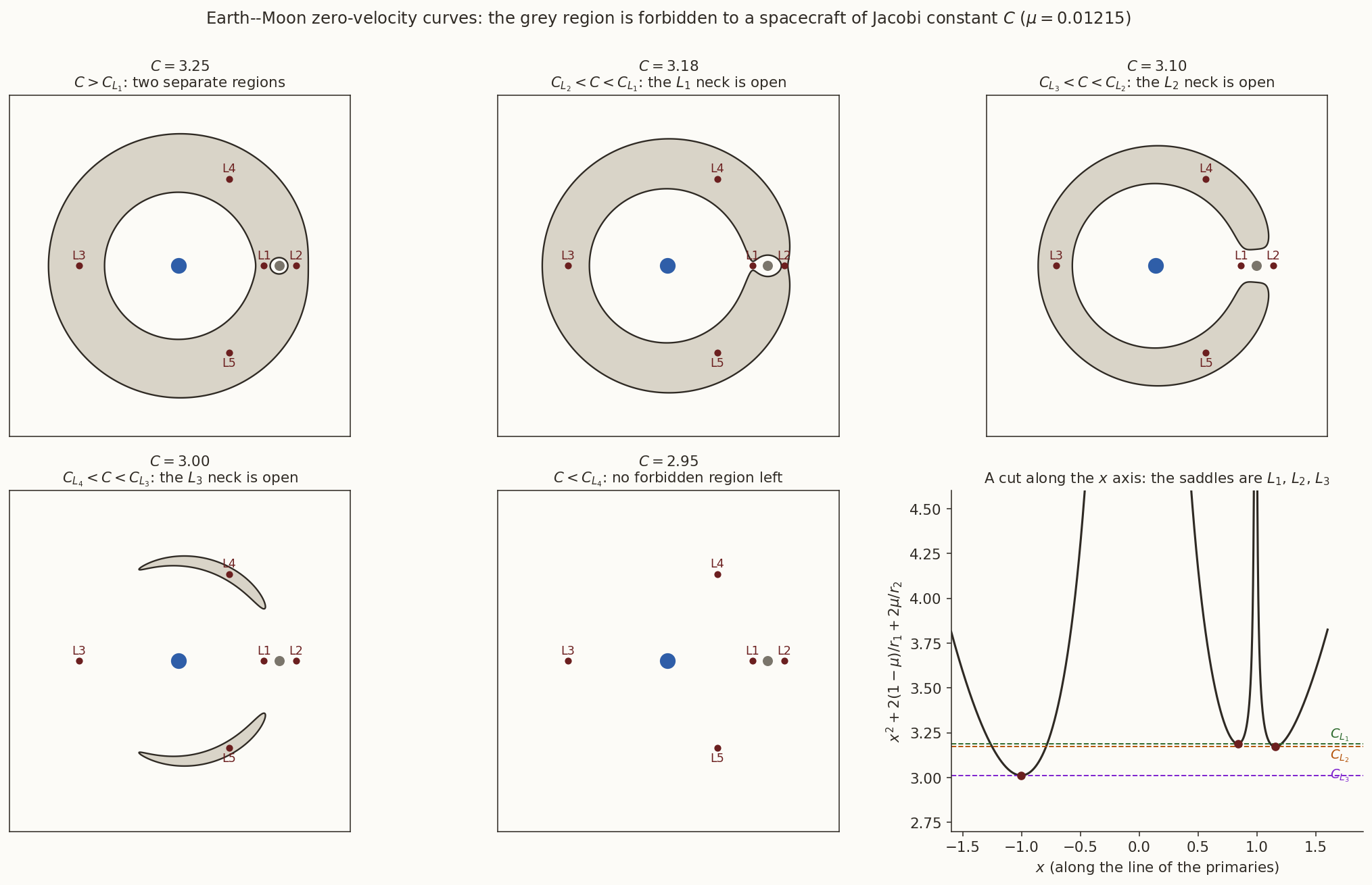
This is the main use of the Jacobi constant. It is a rigorous statement about where the spacecraft cannot go. The Jacobi constants of the equilibrium points (Table 2 below) are the thresholds. For \(C>C_{L_1}\) the Earth region and the Moon region are separated by a wall: a spacecraft in lunar orbit cannot reach the Earth, however it coasts, and a transfer needs a burn that lowers \(C\). For \(C_{L_2}<C<C_{L_1}\) the \(L_1\) neck is open, and a transfer is allowed: the spacecraft is not forbidden to cross, though the dynamics need not take it there.
A spacecraft is at perigee \(300\) km above the Earth, on the Earth–Moon line on the side towards the Moon, moving prograde (so in the \(+y\) direction). What perigee speed (inertial) makes \(C=C_{L_1}\), so that the \(L_1\) neck just opens? Compare with the escape speed and with the perigee speed of a Hohmann transfer to the Moon’s distance.
What you should find
The rotating-frame speed is the inertial speed minus \(n\,r_p\), with \(n=2.6653\times10^{-6}\) rad/s, so \(v_{\rm rot}=v_{\rm in}-0.0178\) km/s. Solving \(C=C_{L_1}=3.1883\) gives \(v_{\rm in}=10.79\) km/s. That is below the escape speed (\(10.926\) km/s) and just below the Hohmann perigee speed to the Moon’s distance (\(10.83\) km/s): the neck at \(L_1\) is closer than the Moon, and the Moon’s pull helps.3 The five equilibrium points
An equilibrium point is a point where a spacecraft at rest in the rotating frame stays at rest: \(\dot{\mathbf r}=\ddot{\mathbf r}=0\), so \(\Omega_x=\Omega_y=\Omega_z=0\), which says that the gravitational pull of the primaries exactly provides the centripetal force that the rotation needs. There are five.
3.1 The triangular points
Look first for points off the axis, \(y\ne0\). The condition \(\Omega_z=0\) gives \(z=0\). The condition \(\Omega_y=0\), divided by \(y\), gives
\[ 1=\frac{1-\mu}{r_1^{3}}+\frac{\mu}{r_2^{3}} . \]
Substituting this “1” into \(\Omega_x=0\),
\[ \Omega_x=x\left[\frac{1-\mu}{r_1^{3}}+\frac{\mu}{r_2^{3}}\right]-\frac{(1-\mu)(x+\mu)}{r_1^{3}}-\frac{\mu(x-1+\mu)}{r_2^{3}} =\mu(1-\mu)\left(\frac1{r_2^{3}}-\frac1{r_1^{3}}\right)=0, \]
so \(r_1=r_2\), and then the first condition gives \(r_1=r_2=1\). The third body is at the same distance from both primaries as they are from each other: the three bodies form an equilateral triangle. There are two such points, one on each side of the axis:
\[ \boxed{\ L_{4,5}=\left(\tfrac12-\mu,\ \pm\tfrac{\sqrt3}{2},\ 0\right)\ } \tag{4}\]
(Figure 2, left). They exist for every \(\mu\), and their position does not depend on the masses at all, in these units.
3.2 The collinear points
On the axis (\(y=z=0\)) only the \(x\) equation is left:
\[ f(x)\equiv x-\frac{(1-\mu)(x+\mu)}{|x+\mu|^{3}}-\frac{\mu(x-1+\mu)}{|x-1+\mu|^{3}}=0 . \tag{5}\]
This is a quintic in disguise. \(f\) goes to \(\mp\infty\) at each primary and \(\pm\infty\) at infinity, so there is exactly one root in each of the three intervals outside the singularities: \(L_1\) between the primaries, \(L_2\) beyond the small one, and \(L_3\) beyond the large one. They are found numerically (a bracketed root-finder is enough).
An estimate near the small primary. Let the distance of \(L_1\) (or \(L_2\)) from \(m_2\) be \(\gamma\), small when \(\mu\) is small. Take \(L_1\), with \(x=1-\mu-\gamma\). In Equation 5, the first two terms are \((1-\mu-\gamma)-(1-\mu)(1-\gamma)^{-2}\approx-3\gamma\) (the centrifugal term contributes \(-\gamma\) and the large primary’s field gradient \(-2\gamma\): together exactly the “tidal plus centrifugal” combination of a rotating frame). The third term is \(-\mu(-\gamma)/\gamma^{3}=+\mu/\gamma^{2}\), the pull of the small primary. Balancing them,
\[ -3\gamma+\frac{\mu}{\gamma^{2}}=0\quad\Longrightarrow\quad \boxed{\ \gamma\approx\left(\frac{\mu}{3}\right)^{1/3}\ } \tag{6}\]
the Hill radius in these units (the same result holds for \(L_2\) at leading order). Sun–Earth: \((3.0404\times10^{-6}/3)^{1/3}=0.0100447\) AU \(=1.5027\times10^{6}\) km, against the exact \(L_1\) at \(1.4976\times10^{6}\) km and \(L_2\) at \(1.5077\times10^{6}\) km, so the Hill value is the average of the two, to the accuracy of the approximation. This is the “\(1.5\) million km” of every description of SOHO, JWST and Aditya-L1.
For the Earth–Moon system (\(\mu=0.0121506\)) find \(L_1\) and \(L_2\) numerically from Equation 5, express their distances from the Moon in km, and compare with Equation 6.
What you should find
\(L_1\) is at \(x=0.836915\) and \(L_2\) at \(x=1.155682\) (and \(L_3\) at \(-1.005063\)). The distances from the Moon are \(\gamma_1=0.150934\) and \(\gamma_2=0.167833\) in units of \(384\,400\) km, i.e. \(58\,019\) km and \(64\,515\) km. The Hill estimate is \((\mu/3)^{1/3}=0.159401\), i.e. \(61\,274\) km, which is the average of \(\gamma_1\) and \(\gamma_2\) (\(0.159384\)) to \(0.01\%\), though each is \(5\%\) away because \(\mu\) is not very small. \(L_1\) is \(326\,381\) km from the Earth.| Earth–Moon | Sun–(Earth+Moon) | |
|---|---|---|
| \(L_1\) (\(x\)) | \(0.836915\) | \(0.989986\) |
| \(L_2\) (\(x\)) | \(1.155682\) | \(1.010075\) |
| \(L_3\) (\(x\)) | \(-1.005063\) | \(-1.000001\) |
| distance of \(L_1\) from the small primary | \(58\,019\) km | \(1\,497\,621\) km |
| distance of \(L_2\) from the small primary | \(64\,515\) km | \(1\,507\,683\) km |
| \(C_{L_1}\) | \(3.188341\) | \(3.000898\) |
| \(C_{L_2}\) | \(3.172160\) | \(3.000894\) |
| \(C_{L_3}\) | \(3.012147\) | \(3.000003\) |
| \(C_{L_4}=C_{L_5}\) (\(=3-\mu(1-\mu)\)) | \(2.987997\) | \(2.999997\) |
4 Stability of the equilibrium points
A spacecraft placed near an equilibrium point either stays near it (stable) or drifts away (unstable). To tell, write \(\mathbf r=\mathbf r_{\rm eq}+\boldsymbol\xi\) in Equation 1 and keep the terms linear in \(\boldsymbol\xi=(\xi,\eta,\zeta)\):
\[ \ddot\xi-2\dot\eta=\Omega_{xx}\xi+\Omega_{xy}\eta,\qquad \ddot\eta+2\dot\xi=\Omega_{xy}\xi+\Omega_{yy}\eta,\qquad \ddot\zeta=\Omega_{zz}\zeta, \]
with the second derivatives of \(\Omega\) evaluated at the point (\(\Omega_{xz}=\Omega_{yz}=0\) there, since \(z=0\)). For solutions \(e^{\lambda t}\) the planar pair gives the characteristic equation
\[ \lambda^{4}+\bigl(4-\Omega_{xx}-\Omega_{yy}\bigr)\lambda^{2}+\Omega_{xx}\Omega_{yy}-\Omega_{xy}^{2}=0 . \tag{7}\]
4.1 The collinear points are unstable
On the axis \(\Omega_{xy}=0\), and with
\[ c_2=\frac{\mu}{|x-1+\mu|^{3}}+\frac{1-\mu}{|x+\mu|^{3}} \tag{8}\]
the second derivatives are \(\Omega_{xx}=1+2c_2\), \(\Omega_{yy}=1-c_2\) and \(\Omega_{zz}=-c_2\). Then Equation 7 becomes
\[ \lambda^{4}+(2-c_2)\lambda^{2}+(1+c_2-2c_2^{2})=0 . \]
Because \(c_2>1\) at the collinear points (it is \(5.15\) at the Earth–Moon \(L_1\) and \(4.06\) at the Sun–Earth \(L_1\)), the constant term is negative, so the quadratic in \(\lambda^{2}\) has one positive and one negative root: two real eigenvalues \(\pm\lambda\), and a pair of imaginary ones \(\pm i\nu\). The out-of-plane motion is \(\ddot\zeta=-c_2\zeta\), a harmonic oscillation of frequency \(\nu_z=\sqrt{c_2}\). So each collinear point is a saddle \(\times\) centre \(\times\) centre: a spacecraft near it oscillates in the plane at \(\nu\) and out of the plane at \(\nu_z\), and any component along the unstable direction grows like \(e^{\lambda t}\).
| \(c_2\) | \(\lambda\) | e-folding time | \(\nu\) (planar) | \(\nu_z\) (vertical) | |
|---|---|---|---|---|---|
| Earth–Moon \(L_1\) | \(5.1476\) | \(2.9321\) | \(1.48\) d | \(2.3344\) | \(2.2688\) |
| Earth–Moon \(L_2\) | \(3.1904\) | \(2.1587\) | \(2.01\) d | \(1.8626\) | \(1.7862\) |
| Sun–Earth \(L_1\) | \(4.0611\) | \(2.5327\) | \(22.95\) d | \(2.0865\) | \(2.0152\) |
| Sun–Earth \(L_2\) | \(3.9405\) | \(2.4843\) | \(23.4\) d | \(2.0570\) | \(1.9851\) |
Unstable does not mean useless. The e-folding time at the Sun–Earth \(L_1\) is \(23\) days. A spacecraft at \(L_1\) must correct its orbit every few weeks (Aditya-L1 does, at spacings of \(25\) to \(106\) days), and the corrections are tiny, because the error is caught while it is small. The instability is also an asset: the stable manifold of the orbit is a trajectory that approaches it for free, and the unstable one a path away from it, the basis of low-energy transfers.
Sun–Earth \(L_1\) has e-folding time \(23\) days. A navigation error of \(1\) cm/s in velocity: how big is it after three months?
Answer
The component along the unstable direction grows by \(e^{t/\tau}\) with \(\tau=22.95\) d: after \(91\) days, \(e^{3.97}=53\). A \(1\) cm/s error becomes about \(0.5\) m/s in speed, and a corresponding position error of tens of thousands of km. That is why a halo orbit needs station-keeping, and why the Indian missions problem says so.4.2 The triangular points: stable if \(\mu<0.0385\)
At \(L_4\) we have \(r_1=r_2=1\), \(x+\mu=\tfrac12\), \(x-1+\mu=-\tfrac12\), \(y=\tfrac{\sqrt3}2\), and the second derivatives work out to
\[ \Omega_{xx}=\tfrac34,\qquad\Omega_{yy}=\tfrac94,\qquad\Omega_{xy}=\pm\tfrac{3\sqrt3}{4}(1-2\mu), \]
with the sign \(+\) at \(L_4\) and \(-\) at \(L_5\) (and \(\Omega_{zz}=-1\), so the vertical motion is a plain oscillation at frequency \(1\)). Then \(4-\Omega_{xx}-\Omega_{yy}=1\) and \(\Omega_{xx}\Omega_{yy}-\Omega_{xy}^{2}=\tfrac{27}{16}\bigl[1-(1-2\mu)^{2}\bigr]=\tfrac{27}{4}\mu(1-\mu)\), so Equation 7 reads
\[ \lambda^{4}+\lambda^{2}+\tfrac{27}{4}\mu(1-\mu)=0, \qquad \lambda^{2}=\frac{-1\pm\sqrt{1-27\mu(1-\mu)}}{2}. \tag{9}\]
If \(1-27\mu(1-\mu)\ge0\) both values of \(\lambda^{2}\) are real and negative, so all four \(\lambda\) are imaginary: stable oscillations. If it is negative, \(\lambda^{2}\) is complex, and one of the four roots has a positive real part: unstable. The boundary is \(27\mu(1-\mu)=1\):
\[ \boxed{\ \mu<\mu_{\rm Routh}=\frac{1-\sqrt{23/27}}{2}=0.0385209\ } \tag{10}\]
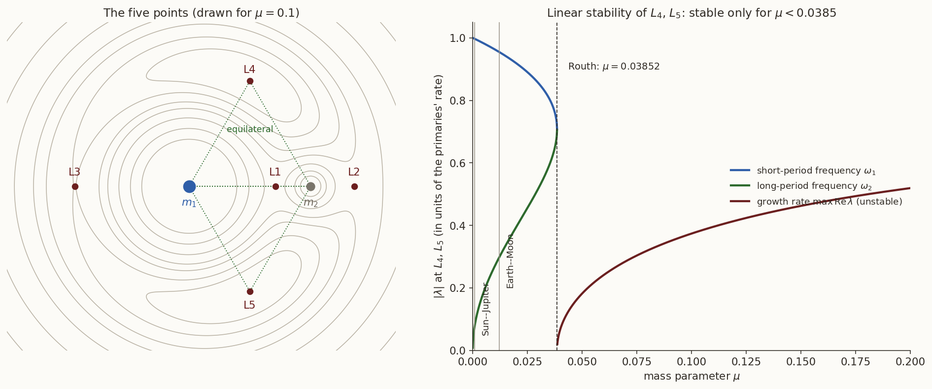
Both Sun–Jupiter (\(\mu=9.54\times10^{-4}\)) and Earth–Moon (\(\mu=0.01215\)) satisfy it. The Trojan asteroids, in the Sun–Jupiter \(L_4\) and \(L_5\) regions, are the standing evidence. The stable oscillations about \(L_4\), \(L_5\) have two frequencies \(\omega_{1,2}=\sqrt{\bigl(1\pm\sqrt{1-27\mu(1-\mu)}\bigr)/2}\): for the Earth–Moon system \(0.9545\) and \(0.2982\), i.e. periods of \(28.6\) and \(91.5\) days. The stability found here is linear, and it holds for the three-body model only: in the real Sun–Earth–Moon system the Sun’s perturbation destabilises the Earth–Moon \(L_4\) and \(L_5\), which is why no swarm of bodies is found there.
Verify that \(L_4\) of Equation 4 satisfies \(\Omega_x=\Omega_y=0\) for any \(\mu\), and find where the discriminant of Equation 9 vanishes. What happens at \(\mu=\tfrac12\) (two equal masses)?
What you should find
At \(L_4\), \(r_1=r_2=1\), so \(\Omega_y/y=1-(1-\mu)-\mu=0\), and with \(x+\mu=\tfrac12\) and \(x-1+\mu=-\tfrac12\), \(\Omega_x=x-\tfrac{1-\mu}{2}+\tfrac\mu2=\bigl(\tfrac12-\mu\bigr)-\tfrac12+\mu=0\). The discriminant vanishes at \(27\mu(1-\mu)=1\), i.e. \(\mu=0.03852\). At \(\mu=\tfrac12\), \(27\mu(1-\mu)=6.75>1\): strongly unstable, with \(\lambda^2=(-1\pm i\sqrt{5.75})/2\).5 Periodic orbits around the collinear points
A spacecraft cannot sit at \(L_1\) exactly (it is unstable), but it can fly around it. The linear solution near a collinear point, with the unstable direction switched off, is a pair of independent oscillations:
\[ \xi=-A_x\cos(\nu t+\phi),\qquad \eta=k\,A_x\sin(\nu t+\phi),\qquad \zeta=A_z\sin(\nu_zt+\psi), \]
where \(\nu\) and \(\nu_z\) are the frequencies of Table 3 and the ratio of the in-plane axes follows from substituting into \(\ddot\xi-2\dot\eta=(1+2c_2)\xi\):
\[ k=\frac{\nu^{2}+1+2c_2}{2\nu} . \tag{11}\]
At the Sun–Earth \(L_1\), \(k=3.229\): the in-plane motion is an ellipse three times longer along the Sun–Earth-perpendicular direction (\(y\)) than along the line to the Sun and Earth (\(x\)). ISRO’s target for Aditya-L1 has \(A_y/A_x=663\,200/209\,200=3.17\).
5.1 Lyapunov orbits
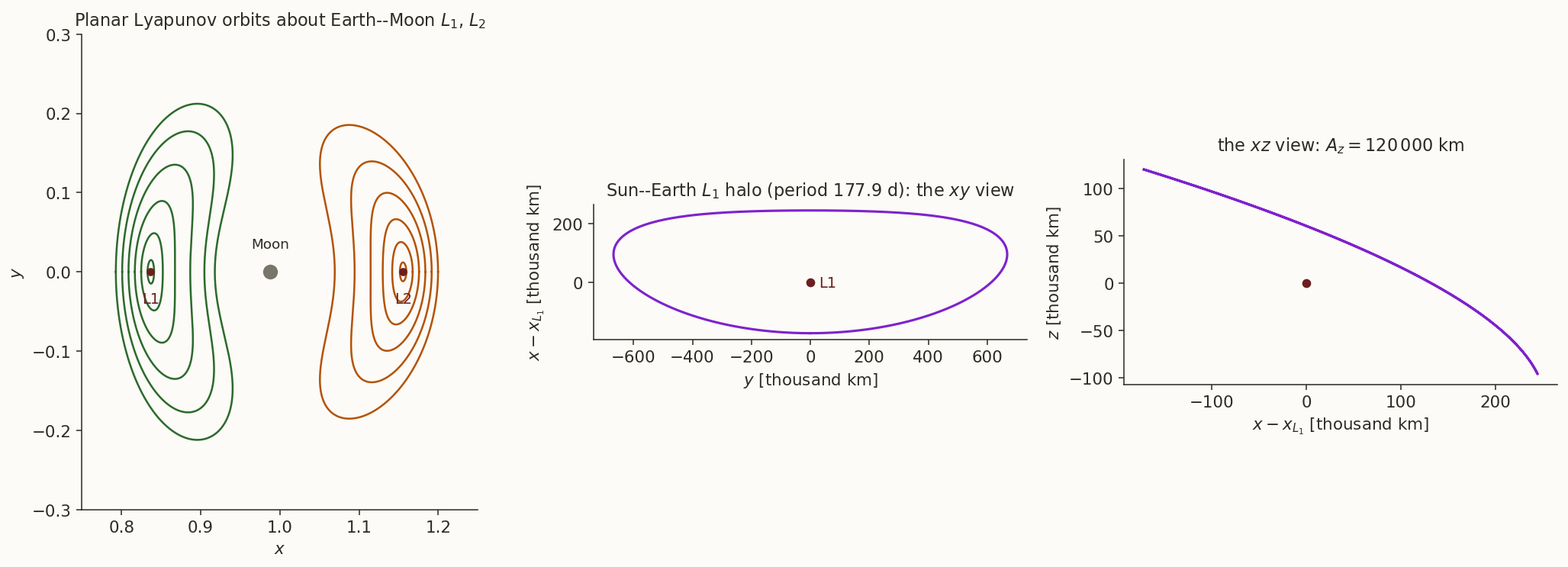
With \(A_z=0\) this is the planar Lyapunov orbit, and its non-linear continuation exists for large amplitudes (Figure 3, left). Its period grows with the amplitude: from \(11.70\) d at small amplitude to \(15.5\) d for the largest drawn about the Earth–Moon \(L_1\).
5.2 Halo orbits
If both \(A_x\) and \(A_z\) are nonzero the linear solution is a quasi-periodic Lissajous curve, unless the two frequencies agree. At the Sun–Earth \(L_1\) they differ slightly, \(\nu=2.0865\) against \(\nu_z=2.0152\) (periods \(175.1\) d and \(181.2\) d). But the non-linear terms make the planar frequency depend on the amplitude, as the growing period of the Lyapunov family shows. At a large enough amplitude the periods meet, and the motion closes into a single periodic three-dimensional curve: a halo orbit (Figure 3, right), named for the way it looks from the Earth, a ring around the Sun. For Aditya-L1’s halo, with \(A_z=120\,000\) km, the computed period is \(177.87\) d, between the two linear periods, and the half-axes are \(A_x=208\,270\) km and \(A_y=667\,997\) km.
How such orbits are computed. The symmetry \((x,y,z,t)\to(x,-y,z,-t)\) of Equation 1 means a periodic orbit that crosses the \(xz\) plane perpendicularly at one point (\(\dot x=\dot z=0\), \(y=0\)) crosses it perpendicularly at the half period too. So only the initial state \((x_0,z_0,\dot y_0)\) needs to be found, with \(z_0\) fixed by the chosen amplitude and the two conditions \(\dot x=\dot z=0\) at the next crossing. A Newton iteration on \((x_0,\dot y_0)\) (single shooting; the script uses a root-finder with finite differences) converges in a few steps from the linear guess. The Jacobi constant is conserved along the result to \(10^{-14}\), which is the first check of any integration.
For the Sun–Earth \(L_1\) (\(c_2=4.0611\)) find \(\lambda\), \(\nu\), \(\nu_z\) and the axis ratio \(k\) from the formulas above. What are the in-plane and out-of-plane periods in days?
What you should find
The characteristic equation \(\lambda^{4}-2.0611\lambda^{2}-27.92=0\) (since \(1+c_2-2c_2^{2}=-27.92\)) gives \(\lambda^{2}=6.4146\) and \(-4.3535\), so \(\lambda=2.5327\) and \(\nu=2.0865\). Also \(\nu_z=\sqrt{4.0611}=2.0152\) and \(k=(4.3535+1+8.1222)/(2\times2.0865)=3.229\). The periods are \(2\pi/\nu=3.0114\) and \(2\pi/\nu_z=3.1179\) time units, i.e. \(175.1\) and \(181.2\) days (one time unit is \(58.132\) d).6 What the restricted problem is used for
- Sun–Earth \(L_1\). SOHO (since 1996) and Aditya-L1 (2023–24) fly halo orbits about the Sun–Earth \(L_1\), where the Sun is always in view and the line to the Earth is short. The Indian missions problems work out why Aditya-L1’s cruise took about \(110\) days and what it cost: insertion \(\Delta v\) against transfer time, the stable manifold, and the instability.
- Sun–Earth \(L_2\). The James Webb Space Telescope flies in an orbit about the Sun–Earth \(L_2\) point, \(1.5077\times10^{6}\) km from the Earth on the far side from the Sun, where the Earth, the Moon and the Sun are all in nearly the same direction, so one sunshield protects the telescope.
- Earth–Moon \(L_2\). A relay satellite in a halo orbit about the Earth–Moon \(L_2\) point can see both the far side of the Moon and the Earth, which a lunar orbiter cannot: the Chinese relay Queqiao (2018) did this for Chang’e 4.
- Low-energy transfers. The unstable and stable manifolds of the periodic orbits are tubes in phase space that carry a spacecraft with little \(\Delta v\) between regions; the Japanese Hiten (1991) used a version of it for its transfer to the Moon.
- Natural bodies. The Trojan asteroids at Jupiter’s \(L_4\) and \(L_5\) points are the natural counterpart of the model. (Faint dust clouds near the Earth–Moon \(L_4\) and \(L_5\), first reported by Kordylewski in 1961, remain a matter of dispute.)
What the model leaves out. (i) The primaries are on circles: the real Earth–Moon orbit has eccentricity \(0.055\) and the Earth’s about the Sun \(0.017\), and the elliptic restricted problem adds a time-dependent term. (ii) For Earth–Moon, the Sun is a fourth body, large enough to destroy the stability of \(L_4\), \(L_5\) and to shift the periodic orbits. (iii) Solar radiation pressure, the Earth’s \(J_2\), and the lumping of Earth and Moon in the Sun–Earth problem. Real mission design therefore uses the CR3BP to find the orbits and manifolds, and then converges them in an ephemeris model with all the real forces.
7 The Hill sphere and the sphere of influence
Equation 6 says \(L_1\) and \(L_2\) sit at the Hill radius \(r_{\rm H}=a\,(m/3M)^{1/3}\) of the small body (of mass \(m\), on a circular orbit of radius \(a\) about the large one of mass \(M\)). Inside it, the small body’s gravity wins against the combined tidal and centrifugal terms of the rotating frame, so a particle can orbit it. For the Earth: \(r_{\rm H}=1.4966\times10^{6}\) km. The sphere of influence of the patched-conics note, \(r_{\rm SOI}=a\,(m/M)^{2/5}=9.25\times10^{5}\) km, is smaller by a factor \(1.6\). They answer different questions. The Hill sphere is where a body can hold on to a satellite in the rotating frame (and so where the equilibrium points are); the sphere of influence is where treating the body as the central one and the other as the disturbance gives the smaller relative perturbation, the criterion that decides where to switch the central body in a patched-conic calculation. The Moon, at \(384\,400\) km, is at \(0.26\) of the Earth’s Hill radius: well inside, as it must be.
In one paragraph. Two primaries on circles and a massless third body, in the rotating frame and in units where the primaries are \(1\) apart and rotate at \(1\), give the equations Equation 1 with the single parameter \(\mu=m_2/(m_1+m_2)\). The Jacobi constant \(C=2\Omega-v^{2}\) is conserved and forbids the spacecraft the regions where \(2\Omega<C\); as \(C\) falls the walls at \(L_1\), \(L_2\), \(L_3\) open in turn. There are five equilibrium points: three collinear ones, from a quintic, and two equilateral ones at \((\tfrac12-\mu,\pm\tfrac{\sqrt3}2)\). The collinear points are unstable saddles with a centre; the triangular ones are stable only for \(\mu<0.0385\). About the collinear points there are periodic orbits, planar (Lyapunov) and three-dimensional (halo), found by shooting, and the Sun–Earth ones are the working orbits of SOHO, JWST and Aditya-L1.
Summary
The numbers of this note are checked by cr3bp-verify.py, using the helper module _cr3bp.py (equations of motion, equilibrium points, linearisation, shooting for Lyapunov and halo orbits); fig-cr3bp.py draws the figures.
Constants used. \(\mu_\oplus=398\,600.4418\) km\(^3\)/s\(^2\), \(\mu_{\rm Moon}=4902.800066\) km\(^3\)/s\(^2\), \(\mu_\odot=1.32712440018\times10^{11}\) km\(^3\)/s\(^2\), \(1\) AU \(=1.495978707\times10^{8}\) km, Moon distance \(384\,400\) km (the full list is on the notation page).
Further reading. V. Szebehely, Theory of Orbits: The Restricted Problem of Three Bodies (Szebehely 1967), is the classical reference; W. S. Koon, M. W. Lo, J. E. Marsden and S. D. Ross, Dynamical Systems, the Three-Body Problem and Space Mission Design (Koon et al. 2011), treats halo orbits, manifolds and low-energy transfers from the viewpoint of the mission designer; C. D. Murray and S. F. Dermott, Solar System Dynamics (Murray and Dermott 1999), chapter 3, is the astronomer’s account; H. D. Curtis, Orbital Mechanics for Engineering Students, has the Lagrange points in the chapter on the restricted problem. D. L. Richardson’s analytic construction of halo orbits is in Celestial Mechanics 22 (1980) 241–253.
Exercises
- Units. Check Table 1: from \(G(m_1+m_2)\) and the distance, compute the time and speed units of the Earth–Moon system. (Answers: \(T=375\,190\) s \(=4.3425\) d; \(1.0245\) km/s.)
- Equilateral points. Show that for \(\mu=\tfrac12\) the triangular points of Equation 4 are at \((0,\pm\tfrac{\sqrt3}2)\), and that the collinear ones are at \(x=0\) (between the equal masses) and symmetric about it. Is the problem then stable at \(L_4\)? (No: \(27\cdot\tfrac14>1\).)
- Collinear point by Newton. Find the Earth–Moon \(L_2\) from Equation 5 starting at \(x=1+\gamma_{\rm Hill}\), and the Sun–Earth \(L_2\) distance from the Earth in km. (Answers: \(x=1.155682\); \(1.5077\times10^{6}\) km.)
- Jacobi constant of a lunar orbit. Find \(C\) for a prograde circular orbit \(100\) km above the Moon’s surface (radius \(1837.4\) km), at four points of the orbit. (Answer: \(C=5.5088\) at all four points, which differ only in the fifth decimal. The orbit is deep inside the Moon’s region, and \(C\gg C_{L_1}=3.188\): to leave it, a burn must lower \(C\) by \(2.3\).)
- Linear analysis. For the Earth–Moon \(L_1\) (\(c_2=5.1476\)) compute \(\lambda\), \(\nu\), \(\nu_z\) and the e-folding time in days. (Answers: \(2.9321\), \(2.3344\), \(2.2688\), \(1.48\) d.)
- Routh. Show that \(\lambda^{4}+\lambda^{2}+\tfrac{27}4\mu(1-\mu)=0\) has purely imaginary roots exactly for \(\mu\le0.0385\), and find the periods of the two motions for Sun–Jupiter (\(\mu=9.54\times10^{-4}\)) in units of Jupiter’s orbital period. (Answers: \(\omega_1=0.99676\) and \(\omega_2=0.08046\), so periods of \(1.003\) and \(12.43\) Jupiter years, i.e. about \(147\) years for the slow libration of the Trojans.)
- Hill and SOI. For the Moon about the Earth (\(m/M=0.01215/0.98785\), \(a=384\,400\) km), compare the Hill radius with the sphere of influence. (Answers: \(r_{\rm H}=61\,500\) km and \(r_{\rm SOI}=66\,200\) km; for a mass ratio this large the SOI is the larger of the two, the opposite of the Earth’s case.)