Relative Motion and the Clohessy–Wiltshire Equations
How a chaser moves near a target on a circular orbit: derivation, solution, geometry and limits
1 Where this note sits
Lambert’s problem (the Lambert note) joins two points anywhere on two orbits, and it is the right tool when the chaser is thousands of kilometres from its target. A few kilometres from the target it is the wrong one, for two reasons.
- Arithmetic. At \(420\) km altitude gravity is \(g=8.625\) m/s\(^2\). A chaser \(10\) km from the target accelerates relative to the target at only \(0.038\) m/s\(^2\): the difference of two vectors of \(8.6\) m/s\(^2\) each, which agree to within \(0.44\%\). Likewise a rendezvous burn of a few m/s is a tiny fraction (one part in \(7700\) per m/s) of the \(7.66\) km/s orbital speed. Everything can be computed, but the answer lives in the last digits of two large numbers.
- Insight. A Lambert solver returns numbers. It does not say why burning forward makes you fall behind, why a radial burn closes after exactly one orbit, or what a given miss distance will cost.
The cure is to describe the chaser relative to the target, in a frame that rotates with the target, and to linearise. The reward is a pair of equations that are linear with constant coefficients and can be solved with sines and cosines. The equations are named after Clohessy and Wiltshire (clohessy1960?), and are Hill’s lunar equations (hill1878?) with the attraction of the body at the origin switched off.
History: two names, 82 years apart. George William Hill (1838–1914) wrote down equations of this form in 1878 for the Moon’s motion relative to the Earth, in a frame turning with the Sun. W. H. Clohessy and R. S. Wiltshire derived them again in 1960 for one spacecraft moving relative to another, with rendezvous guidance in mind. The literature calls them Hill’s, Clohessy–Wiltshire (CW) or Hill–Clohessy–Wiltshire (HCW) equations; here: CW.
Hill worked for the US Nautical Almanac Office from 1861 and spent most of his career at his family farm in West Nyack, New York. Poincaré said that his 1878 memoir contains “the germ of most of the progress” that celestial mechanics has made since.
The route is short, and every step will be done in full:
- The frame (Section 2). Define the target-centred rotating frame and find how fast it turns.
- The exact equation (Section 3). Subtract two two-body equations, and re-express the result in the rotating frame. No approximation has been made yet.
- Linearisation (Section 4). Expand the gravity difference for a nearby chaser. This is the only approximation in the note, and we will do it twice, in two independent ways.
- The solution (Section 5). Integrate in closed form, check the answer by substitution, and package it as a state transition matrix.
- The anatomy of a motion (Section 6). Every solution is a drifting centre carrying a 2:1 epicycle. We find what sets each, and link them to the semi-major axis.
- Worked examples (Section 7) checked against Kepler, and limits of validity (Section 8).
| Symbol | Meaning | Value |
|---|---|---|
| \(\mu\) | Earth’s gravitational parameter | \(398\,600.4418\ \text{km}^3/\text{s}^2\) |
| \(r_t\) | radius of the target’s circular orbit (\(6378.137+420\) km) | \(6798.137\) km |
| \(n=\sqrt{\mu/r_t^{3}}\) | orbital rate of the target, and of the rotating frame | \(1.126378\times10^{-3}\) rad/s |
| \(T=2\pi/n\) | period | \(5578.2\) s \(=92.97\) min |
| \(v_t=nr_t\) | target’s speed | \(7.65727\) km/s |
| \(\boldsymbol\rho=x\hat{\mathbf i}+y\hat{\mathbf j}+z\hat{\mathbf k}\) | chaser’s position relative to the target | |
| \(\mathbf X=(x,\,y,\,\dot x,\,\dot y)^{\mathsf T}\) | in-plane relative state | |
| \(\tau=nt\), \(s=\sin\tau\), \(c=\cos\tau\) | shorthand used in the matrices |
A dot over a symbol means \(d/dt\) as seen in the rotating frame. A derivative taken in the inertial frame carries the subscript \(\mathcal I\).
2 The target-centred rotating frame
2.1 The three axes
At time \(t\) the target is at \(\mathbf r_t\) with velocity \(\mathbf v_t\). Its orbit normal is \(\mathbf h_t=\mathbf r_t\times\mathbf v_t\). Define
\[ \hat{\mathbf i}=\frac{\mathbf r_t}{r_t},\qquad \hat{\mathbf k}=\frac{\mathbf h_t}{h_t},\qquad \hat{\mathbf j}=\hat{\mathbf k}\times\hat{\mathbf i}. \tag{1}\]
These three unit vectors are orthonormal and right-handed (\(\hat{\mathbf i}\times\hat{\mathbf j}=\hat{\mathbf k}\)), and they ride with the target (Figure 1). On a circular orbit the velocity is perpendicular to the radius at every instant, so \(\hat{\mathbf j}\) points along the velocity. The coordinates of the chaser are
- \(x\) — radial: positive means above the target (farther from the Earth);
- \(y\) — along-track: positive means ahead of the target;
- \(z\) — cross-track: out of the orbit plane.
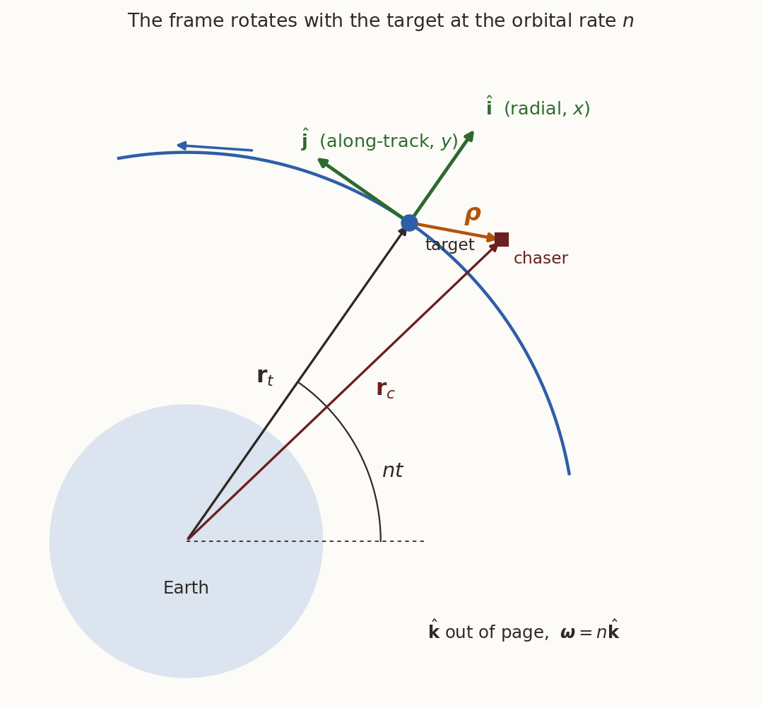
Naming. This frame is called LVLH (local vertical, local horizontal) in NASA documents, RSW or RTN (radial, along-track or transverse, normal) in much of the astrodynamics literature, and the Hill frame in Hill’s honour. Axis conventions differ between sources — NASA’s own LVLH, for example, takes \(x\) roughly along the velocity and \(z\) towards the Earth — so check the axes before using someone else’s matrix. In ISS operations the line along the velocity is the V-bar and the line along the radius vector is the R-bar; an approach along either is a V-bar or an R-bar approach.
To be concrete, choose inertial axes \((X,Y,Z)\) with the orbit in the \(XY\) plane and the target on the \(X\) axis at \(t=0\). The target’s polar angle is then \(nt\), and the unit vectors, written in the inertial basis, are
\[ \hat{\mathbf i}=\begin{pmatrix}\cos nt\\ \sin nt\\ 0\end{pmatrix},\qquad \hat{\mathbf j}=\begin{pmatrix}-\sin nt\\ \cos nt\\ 0\end{pmatrix},\qquad \hat{\mathbf k}=\begin{pmatrix}0\\0\\1\end{pmatrix}. \tag{2}\]
(Check: \(\hat{\mathbf k}\times\hat{\mathbf i}=(0\cdot0-1\cdot\sin nt,\ 1\cdot\cos nt-0\cdot0,\ 0)=\hat{\mathbf j}\), as Equation 1 requires.)
2.2 How fast does the frame turn?
A circular orbit of radius \(r_t\) and angular rate \(n\) needs a centripetal acceleration \(r_tn^2\), and the only force is gravity, \(\mu/r_t^2\). Equating,
\[ r_t\,n^{2}=\frac{\mu}{r_t^{2}}\qquad\Longrightarrow\qquad n=\sqrt{\frac{\mu}{r_t^{3}}}, \tag{3}\]
which is Kepler’s third law for a circle. Now differentiate Equation 2, remembering that \(n\) is a constant:
\[ \begin{aligned} \frac{d\hat{\mathbf i}}{dt}&=n\,(-\sin nt,\ \cos nt,\ 0)^{\mathsf T}=n\,\hat{\mathbf j},\\ \frac{d\hat{\mathbf j}}{dt}&=-n\,(\cos nt,\ \sin nt,\ 0)^{\mathsf T}=-n\,\hat{\mathbf i},\\ \frac{d\hat{\mathbf k}}{dt}&=\mathbf 0 . \end{aligned} \tag{4}\]
All three are of the form \(d\hat{\mathbf e}/dt=\boldsymbol\omega\times\hat{\mathbf e}\) with the angular velocity \(\boldsymbol\omega=n\hat{\mathbf k}\), because \(n\hat{\mathbf k}\times\hat{\mathbf i}=n\hat{\mathbf j}\), \(n\hat{\mathbf k}\times\hat{\mathbf j}=-n\hat{\mathbf i}\) and \(n\hat{\mathbf k}\times\hat{\mathbf k}=\mathbf 0\). So the frame turns about the orbit normal at the constant rate \(n\): once per orbit, \(T=92.97\) min.
2.3 Why a rotating frame at all?
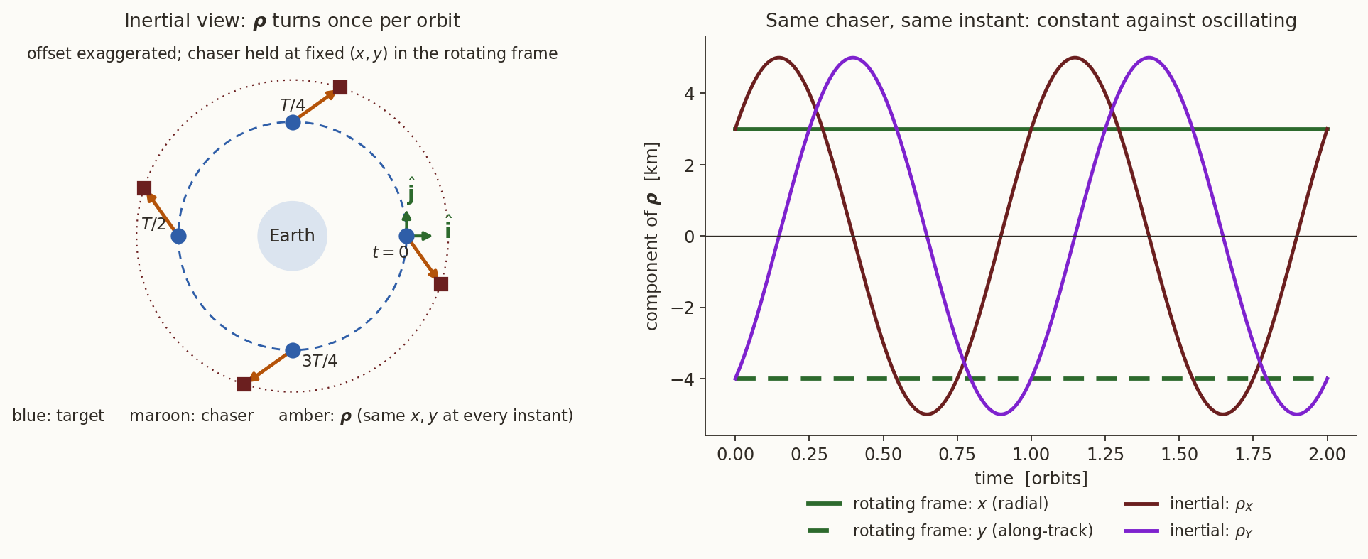
Suppose the chaser sits motionless next to the target: \(3\) km above and \(4\) km behind, say. In the rotating frame its coordinates are \((x,y)=(3,-4)\) km, forever. Seen from an inertial frame, the same offset \(\boldsymbol\rho=x\hat{\mathbf i}+y\hat{\mathbf j}\) has components, from Equation 2,
\[ \rho_X=x\cos nt-y\sin nt,\qquad \rho_Y=x\sin nt+y\cos nt, \]
which swing between \(\pm\sqrt{x^2+y^2}=\pm5\) km once per orbit (Figure 2). The interesting information — how far above, how far ahead — is in the slowly varying rotating-frame numbers; in the inertial frame it is buried in a rotation. This is the first reason to use the rotating frame. The second, which will turn out to matter even more, is that in this frame the target is at rest and the problem has a symmetry (Section 4.4).
3 The exact equation of relative motion
3.1 Subtracting two two-body equations
Let the chaser be at \(\mathbf r_c=\mathbf r_t+\boldsymbol\rho\). Each spacecraft obeys the two-body equation in the inertial frame:
\[ \ddot{\mathbf r}_t=-\frac{\mu\,\mathbf r_t}{r_t^{3}},\qquad \ddot{\mathbf r}_c=-\frac{\mu\,\mathbf r_c}{r_c^{3}} . \]
Subtracting the first from the second, \(\ddot{\boldsymbol\rho}=\ddot{\mathbf r}_c-\ddot{\mathbf r}_t\), gives
\[ \ddot{\boldsymbol\rho}\Big|_{\mathcal I} =-\frac{\mu\,(\mathbf r_t+\boldsymbol\rho)}{|\mathbf r_t+\boldsymbol\rho|^{3}}+\frac{\mu\,\mathbf r_t}{r_t^{3}} . \tag{5}\]
Equation 5 is exact. It used neither the circularity of the target’s orbit nor the smallness of \(\boldsymbol\rho\). It is also useless as it stands, for two reasons: the right-hand side is a difference of two nearly equal vectors (Section 1), and the left-hand side is an acceleration seen from the inertial frame, in which (Section 2.3) the coordinates of \(\boldsymbol\rho\) oscillate even when the chaser is at rest. We fix the second by changing frame, and the first by expanding.
History: where the rotating frame comes from. Gaspard-Gustave Coriolis worked out the complete equations of motion in a rotating frame in 1835 (coriolis1835?), while studying machines with rotating parts, water wheels in particular. He showed that besides the centrifugal term a body moving in the frame feels an acceleration at right angles to its velocity. The name “Coriolis force” came into use only in the early twentieth century. The effect had been used earlier: George Hadley (1735) explained the trade winds by the Earth’s rotation, and Foucault’s pendulum (1851) made it visible.
3.2 Differentiating in a rotating frame, component by component
Write \(\boldsymbol\rho=x\hat{\mathbf i}+y\hat{\mathbf j}\) (the \(z\) axis is treated in Section 4.5). Both the coordinates \(x(t)\), \(y(t)\) and the unit vectors change with time, so the product rule gives two terms for every derivative. Using Equation 4, \(\dot{\hat{\mathbf i}}=n\hat{\mathbf j}\) and \(\dot{\hat{\mathbf j}}=-n\hat{\mathbf i}\):
First derivative.
\[ \begin{aligned} \dot{\boldsymbol\rho}\Big|_{\mathcal I} &=\dot x\,\hat{\mathbf i}+\dot y\,\hat{\mathbf j}+x\,\frac{d\hat{\mathbf i}}{dt}+y\,\frac{d\hat{\mathbf j}}{dt}\\ &=\dot x\,\hat{\mathbf i}+\dot y\,\hat{\mathbf j}+nx\,\hat{\mathbf j}-ny\,\hat{\mathbf i}\\ &=(\dot x-ny)\,\hat{\mathbf i}+(\dot y+nx)\,\hat{\mathbf j}. \end{aligned} \tag{6}\]
Second derivative. Differentiate Equation 6 in the same way. The coefficient of \(\hat{\mathbf i}\) is \((\dot x-ny)\), with derivative \((\ddot x-n\dot y)\) and, from the moving \(\hat{\mathbf i}\), an extra \((\dot x-ny)\,n\hat{\mathbf j}\); the coefficient of \(\hat{\mathbf j}\) is \((\dot y+nx)\), with derivative \((\ddot y+n\dot x)\) and, from the moving \(\hat{\mathbf j}\), an extra \(-(\dot y+nx)\,n\hat{\mathbf i}\). Collecting the \(\hat{\mathbf i}\) terms and the \(\hat{\mathbf j}\) terms:
\[ \begin{aligned} \ddot{\boldsymbol\rho}\Big|_{\mathcal I} &=\Big[(\ddot x-n\dot y)-n(\dot y+nx)\Big]\hat{\mathbf i} +\Big[(\ddot y+n\dot x)+n(\dot x-ny)\Big]\hat{\mathbf j}\\[2pt] &=\big(\ddot x-2n\dot y-n^{2}x\big)\hat{\mathbf i}+\big(\ddot y+2n\dot x-n^{2}y\big)\hat{\mathbf j}. \end{aligned} \tag{7}\]
Nothing here is approximate. The terms that would be there if the frame did not turn are \(\ddot x\,\hat{\mathbf i}+\ddot y\,\hat{\mathbf j}\); everything else comes from the rotation.
3.3 The same result from the transport theorem
The computation above is a special case of a general rule. For any vector \(\mathbf q=q_i\hat{\mathbf i}+q_j\hat{\mathbf j}+q_k\hat{\mathbf k}\) expressed in a frame that rotates with angular velocity \(\boldsymbol\omega\),
\[ \frac{d\mathbf q}{dt}\Big|_{\mathcal I} =\underbrace{\dot q_i\hat{\mathbf i}+\dot q_j\hat{\mathbf j}+\dot q_k\hat{\mathbf k}}_{\displaystyle \frac{d\mathbf q}{dt}\big|_{\mathcal R}} +\;q_i\,\boldsymbol\omega\times\hat{\mathbf i}+q_j\,\boldsymbol\omega\times\hat{\mathbf j}+q_k\,\boldsymbol\omega\times\hat{\mathbf k} =\frac{d\mathbf q}{dt}\Big|_{\mathcal R}+\boldsymbol\omega\times\mathbf q . \tag{8}\]
The first step is the product rule with \(\dot{\hat{\mathbf e}}=\boldsymbol\omega\times\hat{\mathbf e}\) (Section 2.2); the second is linearity of the cross product. Apply Equation 8 to \(\mathbf q=\boldsymbol\rho\), and then again to \(\mathbf q=\dot{\boldsymbol\rho}|_{\mathcal I}\), with \(\dot{\boldsymbol\omega}=\mathbf 0\) because the target’s orbit is circular:
\[ \begin{aligned} \dot{\boldsymbol\rho}\Big|_{\mathcal I}&=\dot{\boldsymbol\rho}+\boldsymbol\omega\times\boldsymbol\rho,\\ \ddot{\boldsymbol\rho}\Big|_{\mathcal I}&=\big(\ddot{\boldsymbol\rho}+\boldsymbol\omega\times\dot{\boldsymbol\rho}\big)+\boldsymbol\omega\times\big(\dot{\boldsymbol\rho}+\boldsymbol\omega\times\boldsymbol\rho\big) =\ddot{\boldsymbol\rho}+2\,\boldsymbol\omega\times\dot{\boldsymbol\rho}+\boldsymbol\omega\times(\boldsymbol\omega\times\boldsymbol\rho). \end{aligned} \]
For \(\boldsymbol\omega=n\hat{\mathbf k}\) and \(\boldsymbol\rho=x\hat{\mathbf i}+y\hat{\mathbf j}\), with \(\hat{\mathbf k}\times\hat{\mathbf i}=\hat{\mathbf j}\) and \(\hat{\mathbf k}\times\hat{\mathbf j}=-\hat{\mathbf i}\):
\[ \begin{aligned} \boldsymbol\omega\times\boldsymbol\rho&=n(x\hat{\mathbf j}-y\hat{\mathbf i}),\\ \boldsymbol\omega\times\dot{\boldsymbol\rho}&=n(\dot x\hat{\mathbf j}-\dot y\hat{\mathbf i}),\\ \boldsymbol\omega\times(\boldsymbol\omega\times\boldsymbol\rho)&=n^{2}\,\hat{\mathbf k}\times(x\hat{\mathbf j}-y\hat{\mathbf i})=-n^{2}(x\hat{\mathbf i}+y\hat{\mathbf j}). \end{aligned} \]
Substituting reproduces Equation 7 line for line. In this language the two extra terms have names: \(2\boldsymbol\omega\times\dot{\boldsymbol\rho}\) is the Coriolis acceleration, and \(\boldsymbol\omega\times(\boldsymbol\omega\times\boldsymbol\rho)=-n^2\boldsymbol\rho\) is the centripetal one. Moved to the other side of the equation of motion they appear as the familiar apparent forces: the Coriolis term \(-2\boldsymbol\omega\times\dot{\boldsymbol\rho}\) (at right angles to the relative velocity, so it does no work) and the centrifugal term \(+n^2\boldsymbol\rho\) (directed away from the Earth’s centre).
3.4 The exact equations in the rotating frame
In LVLH components the target is at \(\mathbf r_t=r_t\hat{\mathbf i}\) and the chaser at \(\mathbf r_t+\boldsymbol\rho=(r_t+x)\hat{\mathbf i}+y\hat{\mathbf j}\), so \(|\mathbf r_t+\boldsymbol\rho|^2=(r_t+x)^2+y^2\equiv\rho_c^{\,2}\). Equate Equation 7 with the right-hand side of Equation 5, component by component, and use \(\mu/r_t^2=n^2r_t\) from Equation 3:
\[ \begin{aligned} \ddot x-2n\dot y-n^{2}x&=-\frac{\mu\,(r_t+x)}{\rho_c^{3}}+n^{2}r_t,\\[2pt] \ddot y+2n\dot x-n^{2}y&=-\frac{\mu\,y}{\rho_c^{3}} . \end{aligned} \tag{9}\]
These are the exact (nonlinear) equations of planar relative motion about a circular reference orbit. We will use them as the “truth” against which CW is judged in Section 8. All that remains is to simplify the right-hand side.
4 Linearisation
4.1 Small parameters and the binomial series
Measure the offset in units of the orbit radius: \(\varepsilon=x/r_t\) and \(\eta=y/r_t\), both small. Then \(\rho_c^{2}=r_t^{2}D\), with
\[ D=(1+\varepsilon)^{2}+\eta^{2}=1+2\varepsilon+\varepsilon^{2}+\eta^{2}. \]
Using \(\mu=n^{2}r_t^{3}\) again, the right-hand sides of Equation 9, divided by \(n^{2}r_t\), are
\[ \frac{\text{RHS}_x}{n^{2}r_t}=1-\frac{1+\varepsilon}{D^{3/2}},\qquad \frac{\text{RHS}_y}{n^{2}r_t}=-\frac{\eta}{D^{3/2}} . \]
Look at the first of these. The “\(1\)” is the target’s own gravity and the second term is the chaser’s: at \(\varepsilon=\eta=0\) they cancel exactly. What survives is the first correction in \(\varepsilon\) and \(\eta\), and this is why a numerical difference of two large accelerations loses digits, while an algebraic expansion does not.
To expand \(D^{-3/2}\) we need the binomial series, valid for \(|u|<1\):
\[ (1+u)^{-3/2}=1-\tfrac32\,u+\tfrac{15}{8}\,u^{2}-\tfrac{35}{16}\,u^{3}+\cdots, \tag{10}\]
(the coefficient of \(u^k\) is \(\binom{-3/2}{k}\); for example \(\binom{-3/2}{2}=\tfrac{(-3/2)(-5/2)}{2}=\tfrac{15}{8}\)). Here \(u=2\varepsilon+\varepsilon^{2}+\eta^{2}\), which is of first order in the small quantities because of the \(2\varepsilon\). Keeping only first-order terms, \(u\approx2\varepsilon\), so
\[ D^{-3/2}\approx1-3\varepsilon . \]
Then
\[ \begin{aligned} \frac{\text{RHS}_x}{n^{2}r_t}&\approx1-(1+\varepsilon)(1-3\varepsilon)\ \to\ 2\varepsilon,\\ \frac{\text{RHS}_y}{n^{2}r_t}&\approx-\eta\,(1-3\varepsilon)\ \to\ -\eta, \end{aligned} \]
where the arrows mean “discard terms of second order”: multiplying out \((1+\varepsilon)(1-3\varepsilon)\) produces an \(\varepsilon^2\) that is not meaningful, since we dropped second-order terms from \(D^{-3/2}\) itself. Multiplying by \(n^{2}r_t\) and returning to \(x=r_t\varepsilon\), \(y=r_t\eta\):
\[ \text{RHS}\;\approx\;\big(2n^{2}x,\ -n^{2}y\big). \tag{11}\]
4.2 Second route: the gravity-gradient tensor
Equation 11 can be reached without expanding anything, and the second derivation shows what it means. Gravity is a vector field \(\mathbf a(\mathbf r)=-\mu\mathbf r/r^{3}\). The difference between the field at the chaser and at the target is, to first order, the Jacobian of the field times the displacement:
\[ \mathbf a(\mathbf r_t+\boldsymbol\rho)-\mathbf a(\mathbf r_t)\approx\mathsf G\,\boldsymbol\rho,\qquad G_{ij}=\frac{\partial a_i}{\partial r_j}\bigg|_{\mathbf r_t}. \]
Differentiating \(a_i=-\mu\,r_i\,r^{-3}\) with \(\partial r/\partial r_j=r_j/r\) (the product rule, one term for each factor):
\[ \frac{\partial a_i}{\partial r_j}=-\mu\Big[\frac{\delta_{ij}}{r^{3}}-\frac{3\,r_ir_j}{r^{5}}\Big] =\frac{\mu}{r^{3}}\Big(3\,\hat r_i\hat r_j-\delta_{ij}\Big). \]
At the target \(\hat{\mathbf r}=\hat{\mathbf i}\), so \(\hat r_i\hat r_j\) is \(1\) for \(i=j=\) radial and \(0\) otherwise, and \(\mu/r_t^{3}=n^{2}\):
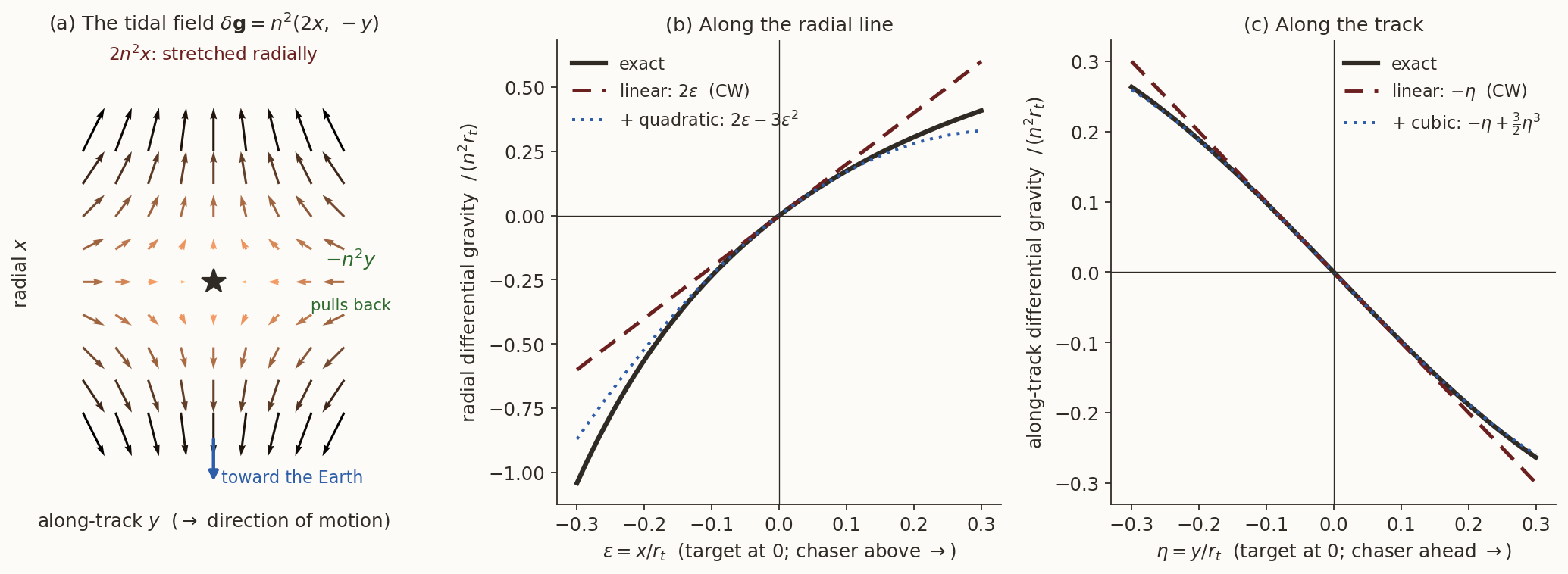
\[ \mathsf G=n^{2}\begin{bmatrix}2&0&0\\0&-1&0\\0&0&-1\end{bmatrix},\qquad \delta\mathbf g=\mathsf G\boldsymbol\rho=n^{2}\,(2x,\ -y,\ -z). \tag{12}\]
The in-plane part is Equation 11. Three things are worth reading off.
- Radial stretch, \(+2n^{2}x\). Gravity falls as \(1/r^{2}\), so a chaser above the target is pulled less than the target. Relative to the target it is left behind, that is, pushed further out. Quantitatively, \(\partial(-\mu/r^{2})/\partial r=+2\mu/r^{3}=2n^{2}\).
- Transverse squeeze, \(-n^{2}y\). Gravity points at the Earth’s centre. A chaser displaced a distance \(y\) along-track sees the centre in a direction rotated by the small angle \(y/r_t\), so it feels a sideways component \(-g\,(y/r_t)=-n^{2}y\) back towards the target’s radial line.
- Zero trace. \(2-1-1=0\): the field is divergence-free (\(\nabla\cdot\mathbf a=0\) in empty space, Laplace’s equation), so a small ring of test masses is stretched in one direction exactly as fast as it is squeezed in the other two (Figure 3, panel a).
History: tides and the 3. Newton’s Principia (1687) explained the ocean tides as the difference between the Moon’s pull on the near side, the centre and the far side of the Earth (Newton 1687). That difference is exactly the gravity gradient of this section. Édouard Roche (1848) used it to show that a body held together only by its own gravity cannot survive inside a critical distance of a planet: the Roche limit.
Hill’s lunar problem turns the same tidal term into the Hill sphere: the distance \(r_H=(\mu_0/3n^{2})^{1/3}\) at which the pull of a body of parameter \(\mu_0\) equals the \(3n^{2}x\) of Equation 13 below. The 3 is ours.
4.3 The Clohessy–Wiltshire equations
Equate Equation 7 with Equation 11:
\[ \ddot x-2n\dot y-n^{2}x=2n^{2}x,\qquad \ddot y+2n\dot x-n^{2}y=-n^{2}y . \]
In the second equation \(-n^{2}y\) appears on both sides and cancels. In the first, move \(n^{2}x\) to the right: \(2n^{2}x+n^{2}x=3n^{2}x\). The result is
\[ \boxed{\ \ddot x-2n\dot y-3n^{2}x=0, \qquad \ddot y+2n\dot x=0 .\ } \tag{13}\]
History: Hill’s equations with the Earth removed. Hill’s lunar equations, in a frame turning at the Sun’s mean motion \(n\), with the origin at the Earth and \(x\) along the Sun–Earth line, read \[\ddot x-2n\dot y-3n^{2}x=-\frac{\mu_0\,x}{r^{3}},\qquad \ddot y+2n\dot x=-\frac{\mu_0\,y}{r^{3}},\] where \(\mu_0\) is the gravitational parameter of the body at the origin and \(r^2=x^2+y^2\). Remove the right-hand sides, the attraction of the body at the origin, and you have Equation 13. The CW equations are Hill’s equations for a target of negligible mass, with the Earth in the role of Hill’s Sun.
Hill’s form is the more general one: put \(\mu_0\) back and the radial line has equilibria at \(x=\pm(\mu_0/3n^{2})^{1/3}\), the Hill sphere.
4.4 Reading the equations
- Linear, with constant coefficients. Both facts come from the same two assumptions: a circular target (constant \(n\)) and a nearby chaser (linearised gravity). This is what makes closed-form solution possible.
- The \(-3n^{2}x\) is a net term. It is \(2n^{2}x\) of gravity gradient plus \(n^{2}x\) of centrifugal acceleration. The two are of the same order, which is why a rotating frame and the tide must be treated together.
- Coupled through Coriolis. The \(x\) equation contains \(\dot y\) and the \(y\) equation contains \(\dot x\): radial motion drives along-track acceleration and vice versa. This coupling is the origin of every counter-intuitive result in rendezvous.
- \(y\) never appears undifferentiated. Neither equation contains \(y\) itself, only \(\dot y\) and \(\ddot y\). Shifting the chaser along the orbit by any amount \(y_0\) changes nothing: every point of the circular orbit is equivalent, which is the symmetry of the problem. It is also the reason a first integral exists (Section 4.6).
- No damping. The equations conserve energy-like quantities (Section 4.6); there is no friction, so no solution decays.
4.5 Out of the plane
For the \(\hat{\mathbf k}\) component, \(\boldsymbol\omega\parallel\hat{\mathbf k}\) gives \(\boldsymbol\omega\times(z\hat{\mathbf k})=\mathbf 0\) and \(\boldsymbol\omega\times(\dot z\hat{\mathbf k})=\mathbf 0\), so the kinematics contributes only \(\ddot z\). The gravity difference contributes \(-n^{2}z\) from Equation 12 (the chaser’s gravity points at the Earth’s centre, which is tilted by \(z/r_t\) from the target’s). Hence
\[ \ddot z+n^{2}z=0 \qquad\Longrightarrow\qquad z(t)=z_0\cos nt+\frac{\dot z_0}{n}\sin nt . \tag{14}\]
A simple harmonic oscillator at the orbital frequency, decoupled from \(x\) and \(y\). Physically it is just a slightly inclined orbit: two orbits of different inclination cross twice per revolution. We stay in-plane from here on.
4.6 Two first integrals
A first integral is a combination of the unknowns and their first derivatives that stays constant. Two exist, and each tells us something without solving anything.
The momentum integral. The second CW equation is an exact derivative:
\[ \ddot y+2n\dot x=\frac{d}{dt}\big(\dot y+2nx\big)=0, \]
so that
\[ \dot y+2nx=\dot y_0+2nx_0\equiv K . \tag{15}\]
What is \(K\)? Compute the chaser’s angular momentum about the Earth’s centre in the inertial frame. Its position is \((r_t+x)\hat{\mathbf i}+y\hat{\mathbf j}\) and, by Equation 6, its velocity is \(\mathbf v_t+\dot{\boldsymbol\rho}|_{\mathcal I}=(\dot x-ny)\hat{\mathbf i}+(nr_t+\dot y+nx)\hat{\mathbf j}\). The \(\hat{\mathbf k}\) component of the cross product is
\[ \begin{aligned} h_c&=(r_t+x)(nr_t+\dot y+nx)-y(\dot x-ny)\\ &=nr_t^{2}+r_t(\dot y+2nx)+\big[x\dot y-y\dot x+n(x^{2}+y^{2})\big]. \end{aligned} \]
The target has \(h_t=nr_t^{2}\). So \(h_c-h_t=r_t(\dot y+2nx)+(\text{second order})\). Each spacecraft conserves its own angular momentum exactly, so \(h_c-h_t\) is exactly constant, and to first order \(K=(h_c-h_t)/r_t\): the momentum integral is the linearised statement that the chaser’s angular momentum, relative to the target’s, is conserved. It is what makes along-track and radial motion inseparable: you cannot change \(\dot y\) without paying for it in \(x\), and the reverse.
The Jacobi (energy) integral. Multiply the \(x\) equation by \(\dot x\) and the \(y\) equation by \(\dot y\), and add:
\[ \dot x\ddot x-2n\dot x\dot y-3n^{2}x\dot x\;+\;\dot y\ddot y+2n\dot x\dot y=0 . \]
The two Coriolis terms \(\mp2n\dot x\dot y\) cancel (they are the “does no work” statement), leaving a perfect derivative:
\[ \frac{d}{dt}\Big[\tfrac12\big(\dot x^{2}+\dot y^{2}\big)-\tfrac32n^{2}x^{2}\Big]=0, \]
so that
\[ J=\tfrac12\big(\dot x^{2}+\dot y^{2}\big)-\tfrac32n^{2}x^{2}=\text{const}. \tag{16}\]
History. Jacobi found the analogous constant of motion for the restricted three-body problem in a rotating frame in 1836. Hill used it in 1877–78 to draw curves of zero velocity: closed curves that the Moon cannot cross, which prove, within his model, that the Moon stays bound to the Earth for ever. Equation 16 is the same integral in the limit that Hill’s problem becomes CW.
The two integrals together give the whole radial motion at once. Substitute \(\dot y=K-2nx\) into \(J\):
\[ J=\tfrac12\dot x^{2}+\tfrac12(K-2nx)^{2}-\tfrac32n^{2}x^{2} =\tfrac12\dot x^{2}+\tfrac12n^{2}x^{2}-2nKx+\tfrac12K^{2}. \]
Complete the square, \(\tfrac12n^{2}x^{2}-2nKx=\tfrac12n^{2}\big(x-2K/n\big)^{2}-2K^{2}\), to get
\[ \tfrac12\dot x^{2}+\tfrac12n^{2}\Big(x-\frac{2K}{n}\Big)^{2}=J+\tfrac32K^{2}=\text{const}. \tag{17}\]
This is the energy of a harmonic oscillator of frequency \(n\) centred at \(x_c=2K/n\). We have just proved, without solving anything, that the radial motion oscillates harmonically at the orbital frequency about a centre fixed by \(K\). The tide pulls outward (Section 4.2), and yet \(x\) cannot run away: the Coriolis coupling converts the outward push into along-track velocity, which by \(\dot y+2nx=K\) pushes back.
5 The solution
5.1 Reduction to one equation
The integral Equation 15 gives \(\dot y=K-2nx\) in terms of \(x\) alone. Substitute it into the \(x\) equation of Equation 13:
\[ \ddot x-2n(K-2nx)-3n^{2}x=0 \quad\Longrightarrow\quad \ddot x+n^{2}x=2nK . \]
Define the constant
\[ x_c\equiv\frac{2K}{n}=4x_0+\frac{2\dot y_0}{n}, \tag{18}\]
so that the equation reads \(\ddot x+n^{2}(x-x_c)=0\): a harmonic oscillator, centred at \(x_c\), as Equation 17 said. (The equality on the right of Equation 18 is \(K=\dot y_0+2nx_0\) inserted.)
5.2 The radial motion
The general solution of \(\ddot x+n^{2}(x-x_c)=0\) is a particular solution plus the homogeneous one. A particular solution is the constant \(x=x_c\) (substitute: \(\ddot x=0\) and \(n^{2}(x_c-x_c)=0\)). The homogeneous solutions are \(\cos nt\) and \(\sin nt\). So
\[ x(t)=x_c+C\cos nt+D\sin nt . \]
The two constants come from the initial conditions:
\[ \begin{aligned} x(0)=x_c+C=x_0\ &\Rightarrow\ C=x_0-x_c=-\Big(3x_0+\frac{2\dot y_0}{n}\Big)\equiv-\alpha,\\ \dot x(0)=nD=\dot x_0\ &\Rightarrow\ D=\frac{\dot x_0}{n}\equiv\beta, \end{aligned} \]
where \(\alpha=3x_0+2\dot y_0/n\) and \(\beta=\dot x_0/n\) will keep reappearing. Written out in the form needed for the matrix below (collect the \(x_0\) terms: \(4x_0-3x_0\cos nt\); the \(\dot y_0\) terms: \(\tfrac{2\dot y_0}{n}(1-\cos nt)\)):
\[ \begin{aligned} x(t)&=x_c-\alpha\cos nt+\beta\sin nt\\ &=(4-3\cos nt)\,x_0+\frac{\sin nt}{n}\,\dot x_0+\frac{2(1-\cos nt)}{n}\,\dot y_0 . \end{aligned} \tag{19}\]
5.3 The velocities
Differentiate Equation 19:
\[ \begin{aligned} \dot x(t)&=n\alpha\sin nt+n\beta\cos nt\\ &=3n\sin nt\;x_0+\cos nt\;\dot x_0+2\sin nt\;\dot y_0 . \end{aligned} \tag{20}\]
For \(\dot y\) we do not integrate anything: Equation 15 gives \(\dot y=K-2nx\), and \(K=nx_c/2\). So \(\dot y=K-2n\big(x_c-\alpha\cos nt+\beta\sin nt\big)\). Since \(2nx_c=4K\), this is \(\dot y=-3K+2n\alpha\cos nt-2n\beta\sin nt\). Expand \(K=\dot y_0+2nx_0\) and \(\alpha=3x_0+2\dot y_0/n\):
\[ \begin{aligned} \dot y(t)&=-3(\dot y_0+2nx_0)+(6nx_0+4\dot y_0)\cos nt-2\dot x_0\sin nt\\ &=-6n(1-\cos nt)\,x_0-2\sin nt\;\dot x_0+(4\cos nt-3)\,\dot y_0 . \end{aligned} \tag{21}\]
5.4 The along-track motion
Integrate Equation 21 from \(0\) to \(t\) with \(y(0)=y_0\). The three integrals needed are
\[ \begin{aligned} \int_0^{t}(1-\cos n\tau')\,d\tau'&=t-\frac{\sin nt}{n},\\ \int_0^{t}\sin n\tau'\,d\tau'&=\frac{1-\cos nt}{n},\\ \int_0^{t}(4\cos n\tau'-3)\,d\tau'&=\frac{4\sin nt}{n}-3t . \end{aligned} \]
Hence, term by term,
\[ y(t)=y_0-6n\Big(t-\frac{\sin nt}{n}\Big)x_0-\frac{2(1-\cos nt)}{n}\,\dot x_0+\Big(\frac{4\sin nt}{n}-3t\Big)\dot y_0, \]
which is, with \(-6nt\,x_0+6\sin nt\,x_0=6(\sin nt-nt)\,x_0\),
\[ \begin{aligned} y(t)&=6(\sin nt-nt)\,x_0+y_0\\ &\quad-\frac{2(1-\cos nt)}{n}\,\dot x_0+\frac{4\sin nt-3nt}{n}\,\dot y_0 . \end{aligned} \tag{22}\]
The terms in \(nt\) are the only ones that grow without bound; we will come back to them in Section 6.
5.5 Checking the solution
A derived formula should be checked by an independent route. Take each initial condition on its own (the equations are linear, so contributions add) and substitute into Equation 13. Write \(c=\cos nt\), \(s=\sin nt\).
Unit \(x_0\): \(x=4-3c\), \(y=6(s-nt)\), so \(\ddot x=3n^{2}c\), \(\dot x=3ns\), \(\dot y=6n(c-1)\), \(\ddot y=-6n^{2}s\):
\[ \begin{aligned} \ddot x-2n\dot y-3n^{2}x&=3n^{2}c+12n^{2}(1-c)-3n^{2}(4-3c)\\ &=(3-12+9)\,n^{2}c+(12-12)\,n^{2}=0\ \checkmark\\ \ddot y+2n\dot x&=-6n^{2}s+2n\,(3ns)=0\ \checkmark \end{aligned} \]
Unit \(\dot x_0\): \(x=s/n\), \(y=-2(1-c)/n\), so \(\ddot x=-ns\), \(\dot x=c\), \(\dot y=-2s\), \(\ddot y=-2nc\):
\[ \begin{aligned} \ddot x-2n\dot y-3n^{2}x&=-ns+4ns-3ns=0\ \checkmark\\ \ddot y+2n\dot x&=-2nc+2nc=0\ \checkmark \end{aligned} \]
Unit \(\dot y_0\): \(x=2(1-c)/n\), \(y=(4s-3nt)/n\), so \(\ddot x=2nc\), \(\dot x=2s\), \(\dot y=4c-3\), \(\ddot y=-4ns\):
\[ \begin{aligned} \ddot x-2n\dot y-3n^{2}x&=2nc-2n(4c-3)-6n(1-c)\\ &=(2-8+6)\,nc+(6-6)\,n=0\ \checkmark\\ \ddot y+2n\dot x&=-4ns+4ns=0\ \checkmark \end{aligned} \]
Unit \(y_0\): \(x=0\), \(y=1\) trivially. And the initial conditions: at \(t=0\), \(c=1\), \(s=0\), so Equation 19, Equation 20, Equation 22 and Equation 21 return \(x_0\), \(\dot x_0\), \(y_0\), \(\dot y_0\) (\(\checkmark\)). A last check at small times: expanding \(4-3\cos nt\approx1+\tfrac32n^{2}t^{2}\) and \(2(1-\cos nt)/n\approx nt^{2}\) gives \(\ddot x(0)=3n^{2}x_0+2n\dot y_0\), which is exactly what the first equation of Equation 13 says at \(t=0\). For \(t\ll1/n\) the motion is ballistic, and the first correction is the equation itself. (codes/cw-verify.py repeats all of this symbolically.)
5.6 The state transition matrix
Collect the in-plane state as \(\mathbf X=(x,\ y,\ \dot x,\ \dot y)^{\mathsf T}\). The CW equations are a first-order linear system
\[ \dot{\mathbf X}=\mathsf A\,\mathbf X,\qquad \mathsf A=\begin{bmatrix}0&0&1&0\\0&0&0&1\\3n^{2}&0&0&2n\\0&0&-2n&0\end{bmatrix}, \tag{23}\]
where rows 3 and 4 are the two CW equations solved for \(\ddot x\) and \(\ddot y\). Because the solution is linear in the initial state, it can be written \(\mathbf X(t)=\mathbf\Phi(t)\mathbf X_0\), where the \(j\)-th column of \(\mathbf\Phi\) is the solution that starts from the \(j\)-th unit vector. Reading the columns off Equation 19, Equation 20, Equation 22 and Equation 21 (\(\tau=nt\), \(s=\sin\tau\), \(c=\cos\tau\)):
\[ \mathbf\Phi(t)=\begin{bmatrix}\mathbf\Phi_{rr}&\mathbf\Phi_{rv}\\ \mathbf\Phi_{vr}&\mathbf\Phi_{vv}\end{bmatrix}, \]
\[ \mathbf\Phi_{rr}=\begin{bmatrix}4-3c & 0\\ 6(s-\tau) & 1\end{bmatrix}, \qquad \mathbf\Phi_{rv}=\frac1n\begin{bmatrix}s & 2(1-c)\\ -2(1-c) & 4s-3\tau\end{bmatrix}, \]
\[ \mathbf\Phi_{vr}=\begin{bmatrix}3ns & 0\\ -6n(1-c) & 0\end{bmatrix}, \qquad \mathbf\Phi_{vv}=\begin{bmatrix}c & 2s\\ -2s & 4c-3\end{bmatrix}. \tag{24}\]
(The subscripts \(r\) and \(v\) stand for position \(\mathbf r=(x,y)\) and velocity \(\mathbf v=(\dot x,\dot y)\). For example \(\mathbf\Phi_{rv}\) says how the final position depends on the initial velocity.)
What to know about \(\mathbf\Phi\).
- \(\mathbf\Phi(0)=\mathsf I\). Obvious from the formulas, and what a “transition matrix” must do at zero elapsed time.
- \(\dot{\mathbf\Phi}=\mathsf A\mathbf\Phi\). Each column is a solution of \(\dot{\mathbf X}=\mathsf A\mathbf X\). Formally \(\mathbf\Phi(t)=e^{\mathsf At}\), the matrix exponential.
- Group property, \(\mathbf\Phi(t_1+t_2)=\mathbf\Phi(t_2)\mathbf\Phi(t_1)\). The system is autonomous (the coefficients do not depend on time), and solutions of a linear ODE are unique, so propagating for \(t_1\) and then \(t_2\) is the same as propagating for \(t_1+t_2\). The trigonometry confirms it. For example, the \((\dot x,\dot x)\) entry of \(\mathbf\Phi(t_2)\mathbf\Phi(t_1)\) is row 3 of \(\mathbf\Phi(t_2)\) times column 3 of \(\mathbf\Phi(t_1)\): \[ \begin{aligned} (3ns_2)\frac{s_1}{n}+0+c_2c_1+(2s_2)(-2s_1)&=3s_1s_2+c_1c_2-4s_1s_2\\ &=c_1c_2-s_1s_2=\cos(\tau_1+\tau_2), \end{aligned} \] which is the \((\dot x,\dot x)\) entry of \(\mathbf\Phi(t_1+t_2)\).
- Inverse. \(\mathbf\Phi(t)^{-1}=\mathbf\Phi(-t)\) (the group property with \(t_2=-t_1\)): one matrix multiply also propagates backwards.
- \(\det\mathbf\Phi=1\). For \(\mathbf\Phi=e^{\mathsf At}\), \(\det\mathbf\Phi=e^{t\,\mathrm{tr}\,\mathsf A}\) (Liouville’s formula), and \(\mathrm{tr}\,\mathsf A=0\). Areas in the \((\mathbf r,\mathbf v)\) phase space are preserved: relative motion has no sinks.
- A numerical example. At half an orbit, \(\tau=\pi\), \(c=-1\), \(s=0\), and in the scaled variables \((x,\ y,\ \dot x/n,\ \dot y/n)\) the matrix is \[ \begin{bmatrix}7&0&0&4\\-6\pi&1&-4&-3\pi\\0&0&-1&0\\-12&0&0&-7\end{bmatrix}. \]
History. Peano (1888), and Baker (1905) after him, wrote the solution of a linear differential equation with time-varying coefficients as a series of repeated integrals. With constant coefficients that series sums to the matrix exponential used here. The phrase “state transition” entered engineering with the state-space methods of 1960 — the same year as Clohessy and Wiltshire — when Kalman published his celebrated paper on filtering (kalman1960?).
5.7 Where the drift comes from: the eigenstructure
Why does a linear oscillating system contain a term growing in \(t\)? Look at the eigenvalues of \(\mathsf A\). Expand \(\det(\lambda\mathsf I-\mathsf A)\) along the second column, which has a single non-zero entry \(\lambda\):
\[ \begin{aligned} \det(\lambda\mathsf I-\mathsf A)&=\lambda\,\det\begin{bmatrix}\lambda&-1&0\\-3n^{2}&\lambda&-2n\\0&2n&\lambda\end{bmatrix}\\ &=\lambda\Big[\lambda(\lambda^{2}+4n^{2})-3n^{2}\lambda\Big]=\lambda^{2}(\lambda^{2}+n^{2}). \end{aligned} \tag{25}\]
The eigenvalues are \(\lambda=\pm in\) (simple, giving the oscillation) and \(\lambda=0\) (double). No eigenvalue has a positive real part, so nothing grows exponentially. The double zero is the interesting one. Solving \(\mathsf A\mathbf v=\mathbf 0\) gives only one eigenvector, \(\mathbf v=(0,1,0,0)^{\mathsf T}\) (a pure along-track shift), so \(\mathsf A\) has a Jordan block and a second, generalised eigenvector \(\mathbf w\) with \(\mathsf A\mathbf w=-\tfrac32n\,\mathbf v\):
\[ \mathbf w=\big(1,\ 0,\ 0,\ -\tfrac32n\big)^{\mathsf T}: \qquad \mathsf A\mathbf w=\big(0,\ -\tfrac32n,\ 0,\ 0\big)^{\mathsf T}=-\tfrac32n\,\mathbf v . \]
The solution that starts at \(\mathbf w\) is \(e^{\mathsf At}\mathbf w=\mathbf w+t\,\mathsf A\mathbf w=\big(1,\ -\tfrac32nt,\ 0,\ -\tfrac32n\big)^{\mathsf T}\): the chaser sits \(1\) km higher than the target and drifts steadily backwards at \(\tfrac32n\) per km of altitude. That is a circular orbit at a different radius, whose period differs from the target’s (Section 6.3). So the four fundamental motions are:
| Mode | State | Meaning |
|---|---|---|
| shift | \((0,1,0,0)\) | the same circle, \(1\) km ahead: an equilibrium |
| shear | \((1,\,-\tfrac32nt,\,0,\,-\tfrac32n)\) | a neighbouring circle: steady drift |
| epicycle, 2 modes | \(\cos nt,\ \sin nt\) | the oscillation at frequency \(n\) |
Any chaser motion is a combination of these. The next section shows that picture explicitly, and with the fourth column \(\dot y_0\) of \(\mathbf\Phi\) it recovers the \(-3\dot y_0t\) in Equation 22.
6 The anatomy of a natural motion
6.1 Drift or no drift
The only terms in \(\mathbf\Phi\) that grow without bound are those proportional to \(\tau=nt\), and they all sit in the \(y\) row: \(-6nt\,x_0\) from Equation 22 and \(-3t\,\dot y_0\). Collecting,
\[ y(t)=\underbrace{-3\,(2nx_0+\dot y_0)\,t}_{\text{secular drift}}+\text{bounded terms} =-3K\,t+\text{bounded terms}. \]
Hence relative motion is bounded if and only if \(K=0\):
\[ \boxed{\ \text{Relative motion is bounded}\iff \dot y_0=-2n\,x_0 .\ } \tag{26}\]
The condition says: match the target’s period. We will see in Section 6.3 that \(\dot y_0+2nx_0\) measures the difference in semi-major axis between the chaser’s orbit and the target’s. Any chaser whose along-track velocity differs from \(-2nx_0\) has a different semi-major axis, and drifts.
6.2 Guiding centre and epicycle
Equation 19 and Equation 20 suggest rewriting everything in terms of the constants we met: \(x_c=4x_0+2\dot y_0/n\), \(\alpha=3x_0+2\dot y_0/n\) and \(\beta=\dot x_0/n\). The solution for \(y\), from Equation 22, is
\[ y(t)=y_c-\tfrac32\,n\,x_c\,t+2\alpha\sin nt+2\beta\cos nt,\qquad y_c\equiv y_0-2\beta=y_0-\frac{2\dot x_0}{n}, \]
(to see this, integrate \(\dot y=-3K+2n\alpha\cos nt-2n\beta\sin nt\) from Section 5.3, which gives \(y=y_0-3Kt+2\alpha\sin nt-2\beta(1-\cos nt)\), and use \(K=\tfrac12nx_c\) and \(y_c=y_0-2\beta\)). Now combine \(\alpha=A\cos\phi\), \(\beta=A\sin\phi\), with \(A=\sqrt{\alpha^{2}+\beta^{2}}\). Then \(-\alpha\cos nt+\beta\sin nt=-A\cos(nt+\phi)\) and \(2\alpha\sin nt+2\beta\cos nt=2A\sin(nt+\phi)\), so
\[ \boxed{\begin{aligned}x(t)&=x_c-A\cos(nt+\phi),\\ y(t)&=y_c-\tfrac32\,n\,x_c\,t+2A\sin(nt+\phi).\end{aligned}} \tag{27}\]
Eliminating the phase \(nt+\phi\):
\[ \Big(\frac{x-x_c}{A}\Big)^{2}+\Big(\frac{y-y_c+\tfrac32nx_c\,t}{2A}\Big)^{2}=1 . \]
This says, in words, that every natural motion is a 2:1 ellipse — radial semi-axis \(A\), along-track semi-axis \(2A\), traversed once per orbit — whose centre drifts along-track at the constant speed \(-\tfrac32nx_c\). The four constants \((x_c,\,y_c,\,A,\,\phi)\) are the four initial conditions in a better basis:
| Constant | What it sets | Mode of Table 2 |
|---|---|---|
| \(y_c\) | where the guiding centre starts along-track | shift |
| \(x_c=4x_0+2\dot y_0/n\) | the altitude of the guiding centre, and its drift rate \(-\tfrac32nx_c\) | shear |
| \(A=\sqrt{(3x_0+2\dot y_0/n)^{2}+(\dot x_0/n)^{2}}\) | the size of the epicycle | epicycle |
| \(\phi=\arg(\alpha+i\beta)\) | where on the epicycle the chaser starts | epicycle |
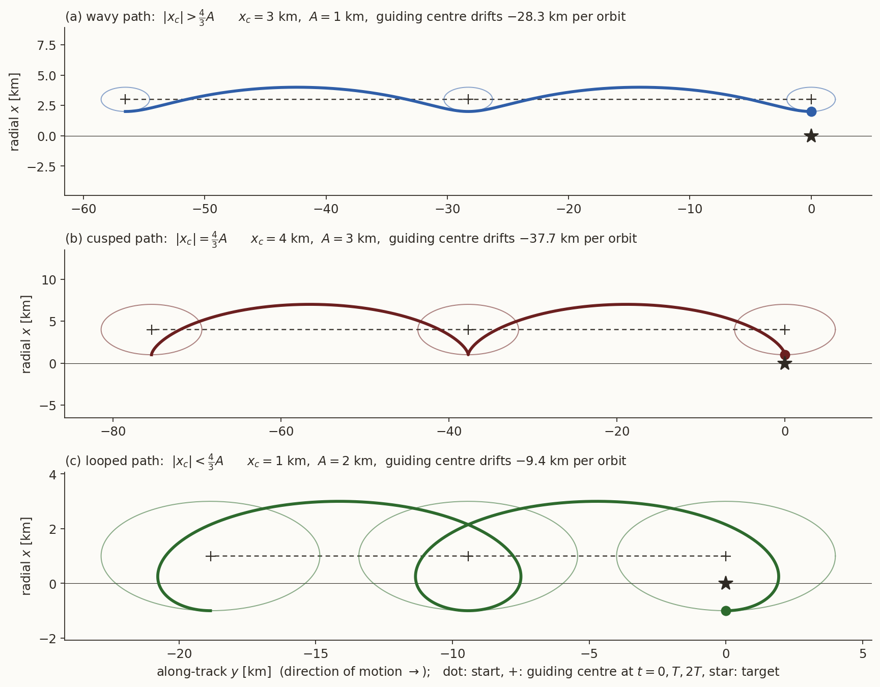
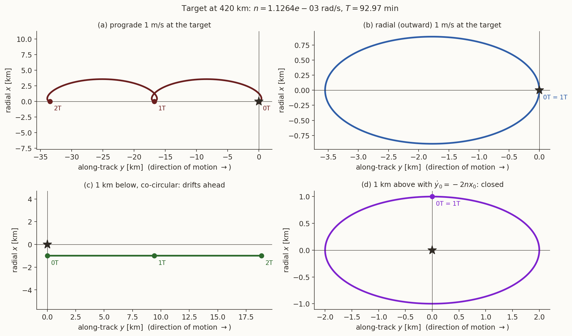
The shape of the track depends on one ratio, \(x_c/A\) (Figure 4). The along-track velocity is \(\dot y=-\tfrac32nx_c+2nA\cos(nt+\phi)\). It changes sign if and only if \(2A>\tfrac32\lvert x_c\rvert\):
- \(\lvert x_c\rvert>\tfrac43A\): \(\dot y\) never changes sign. The path is wavy, always moving the same way along-track.
- \(\lvert x_c\rvert=\tfrac43A\): \(\dot y\) touches zero once per orbit. The path has cusps. (A chaser released from rest above the target, \(\mathbf X_0=(x_0,0,0,0)\), has \(x_c=4x_0\) and \(A=3x_0\), which is exactly this case.)
- \(\lvert x_c\rvert<\tfrac43A\): the path loops.
- \(x_c=0\): no drift, a closed 2:1 ellipse centred on the guiding centre at \(y_c\).
History: epicycles again. The word is Greek astronomy’s: in the Ptolemaic system a planet moves on a small circle (the epicycle) whose centre moves on a larger one (the deferent). The decomposition into a drifting guiding centre and a small oscillation about it is the same idea, and it came back in the twentieth century. The epicyclic approximation of galactic dynamics describes stars on near-circular orbits this way, and the axis ratio \(2\!:\!1\) above is \(2\Omega/\kappa\) with \(\kappa=\Omega\), which holds for a Kepler (inverse-square) force.
Hill’s local approximation, extended to disks, became the shearing sheet used for galactic disks (Goldreich and Lynden-Bell, 1965; Julian and Toomre, 1966) and for planetary rings.
6.3 Why the guiding centre is the difference in semi-major axis
The guiding-centre altitude \(x_c\) has an exact orbital meaning. Compare the specific energies of the chaser and the target, to first order in the offset. The chaser’s inertial speed squared is, using Equation 6,
\[ v_c^{2}=(\dot x-ny)^{2}+(nr_t+\dot y+nx)^{2}\approx n^{2}r_t^{2}+2nr_t(\dot y+nx), \]
and its distance from the Earth is \(|\mathbf r_t+\boldsymbol\rho|\approx r_t+x\), so \(-\mu/|\mathbf r_c|\approx-\mu/r_t+\mu x/r_t^{2}=-\mu/r_t+n^{2}r_tx\). Hence
\[ E_c-E_t\approx nr_t(\dot y+nx)+n^{2}r_tx=nr_t\,(\dot y+2nx)=nr_t\,K . \]
With \(E=-\mu/2a\) we have \(\delta E=\mu\,\delta a/2a^{2}\), so \(\delta a=2a^{2}\,\delta E/\mu=2r_t^{2}\,nr_tK/(n^{2}r_t^{3})\):
\[ \boxed{\ \delta a=\frac{2K}{n}=x_c=4x_0+\frac{2\dot y_0}{n}.\ } \tag{28}\]
The guiding centre sits at the difference of semi-major axes, and the momentum integral \(K\) is the energy difference per unit \(nr_t\) (for neighbouring circular orbits \(\delta E=n\,\delta h\), so the angular-momentum and the energy descriptions of \(K\) agree). Now Kepler’s third law, \(n\propto a^{-3/2}\), gives the chaser’s angular rate \(n+\delta n\) with \(\delta n=-\tfrac32n\,\delta a/r_t\). The chaser’s angular position drifts relative to the target at \(\delta n\), so along-track it drifts at
\[ r_t\,\delta n=-\tfrac32\,n\,\delta a=-\tfrac32\,n\,x_c, \]
exactly the guiding-centre drift in Equation 27. The CW drift is Kepler’s third law: a higher orbit (\(x_c>0\)) is slower and falls behind; a lower one gets ahead. This identity was derived here independently of CW, from energy and Kepler alone, and (codes/cw-verify.py) it holds numerically: for a small test offset the exact \(\Delta a\) from the energy of the chaser agrees with \(x_c\) to six figures.
History. Kepler published the third law in 1619 (Harmonices Mundi) as an empirical regularity of the planets; Newton showed in the Principia (1687) that it follows from an inverse-square force (Newton 1687). Using it to predict how fast two spacecraft drift apart is the same arithmetic Kepler did for the planets, now run for the ISS.
7 Worked examples, checked against Kepler
7.1 Example 1: a 1 m/s prograde burn
Given: the chaser starts at the target, \(\mathbf X_0=(0,\,0,\,0,\,\Delta v)^{\mathsf T}\), with \(\Delta v=1\) m/s \(=10^{-3}\) km/s. Note \(\Delta v/n=0.88780\) km. Only the last column of Equation 24 acts:
\[ x(t)=\frac{2(1-\cos nt)}{n}\,\Delta v, \qquad y(t)=\frac{4\sin nt-3nt}{n}\,\Delta v . \]
At half an orbit \(\tau=\pi\) (\(c=-1\), \(s=0\)) and at a full orbit \(\tau=2\pi\) (\(c=1\), \(s=0\)):
| \(t=T/2\) | \(t=T\) | |
|---|---|---|
| \(x\) [km] | \(4\Delta v/n=\mathbf{3.551}\) | \(0\) |
| \(y\) [km] | \(-3\pi\Delta v/n=-8.367\) | \(-6\pi\Delta v/n=\mathbf{-16.735}\) |
In the language of Section 6.2: \(x_c=2\Delta v/n=1.776\) km, \(A=\alpha=2\Delta v/n=1.776\) km, so the chaser rises from \(0\) to \(2x_c=3.55\) km and the guiding centre drifts \(-3\pi x_c=-3T\Delta v\) per orbit. A convenient memory aid:
\[ \boxed{\ \text{Speeding up makes you fall behind: } 3T\,\Delta v=16.7\ \text{km per orbit per m/s.}\ } \]
History: Gemini 4, June 1965. James McDivitt tried to fly close to the spent Titan II second stage that had put him in orbit. Simply thrusting towards the stage changed his orbit rather than his position relative to it, the stage drew away, and after using almost half his thruster propellant he gave up to concentrate on the spacewalk. The lesson changed how NASA planned rendezvous: later missions approached “upward”, from a lower, faster orbit. The first successful rendezvous was Gemini 6A and 7 in December 1965.
Buzz Aldrin, who flew on Gemini 12, wrote his 1963 MIT doctoral thesis on manned rendezvous guidance (aldrin1963?) and was nicknamed “Dr. Rendezvous”.
7.2 Check against Kepler
Nothing in CW is new physics: it must agree with vis-viva and Kepler’s third law to first order. Here are the numbers by the other route.
Step 1: the new orbit. Vis-viva, \(v^{2}=\mu(2/r-1/a)\), differentiated at fixed \(r\) with \(v=r\,n\) on the circle, gives \(2v\,\delta v=\mu\,\delta a/a^{2}\), so
\[ \Delta a=\frac{2a^{2}v\,\Delta v}{\mu}=\frac{2a\,\Delta v}{v}=\frac{2\Delta v}{n}=1.7756\ \text{km}. \]
(using \(\mu=n^{2}a^{3}\) and \(v=na\).) This equals the CW \(x_c\), as Equation 28 said it must.
Step 2: the far side of the new orbit. The burn point is the new orbit’s pericentre (a burn along the velocity at a circular orbit raises the opposite side), so its apocentre is \(a+2\Delta a\), i.e. \(x=2\Delta a=3.551\) km above the target (\(\checkmark\) the table, at \(t=T/2\)).
Step 3: the period and the lag. \(T\propto a^{3/2}\) gives \(\Delta T=\tfrac32T\,\Delta a/a=\tfrac32(5578.2\ \text{s})(1.7756/6798.137)=2.1855\) s. After one target period the chaser has not completed its longer orbit, so it is behind by \(v\,\Delta T=7.65727\times2.1855=16.735\) km (\(\checkmark\)). Algebraically the two routes are the same number: \(v\,\Delta T=\tfrac32\,v\,T\,\Delta a/a=\tfrac32(na)(2\pi/n)(2\Delta v/n)/a=6\pi\Delta v/n\), which is the table’s \(-6\pi\Delta v/n\).
How good is the first-order theory? Integrating both spacecraft exactly (codes/cw-verify.py):
| CW | exact two-body | |
|---|---|---|
| \(x(T/2)\) [km] | \(3.5512\) | \(3.5472\) |
| \(y(T/2)\) [km] | \(-8.3673\) | \(-8.3673\) |
| \(x(T)\) [km] | \(0\) | \(-0.0206\) |
| \(y(T)\) [km] | \(-16.7347\) | \(-16.7434\) |
The along-track lag after one orbit differs by \(0.05\%\); the neglected terms are of relative order \(\Delta a/a\sim3\times10^{-4}\).
7.3 The co-circular drift
Suppose instead the chaser is on a circular orbit \(1\) km below the target, \(\mathbf X_0=(-1,\,0,\,0,\,\dot y_0)\). What \(\dot y_0\) makes the orbit circular? The chaser’s inertial speed is \(n'(a+x)\) with \(n'=n\,(1+x/a)^{-3/2}\approx n\big(1-\tfrac32x/a\big)\), while the rotating frame, at the same radius, moves at \(n(a+x)\). The difference is the velocity relative to the frame:
\[ \dot y_0=(n'-n)(a+x_0)\approx-\tfrac32\,n\,x_0 . \]
For \(x_0=-1\) km this is \(\dot y_0=+1.690\) m/s (ahead). With this value \(K=\dot y_0+2nx_0=\tfrac12nx_0\), i.e. \(x_c=x_0\): the chaser is its own guiding centre (\(A=3x_0+2\dot y_0/n=0\)), and it drifts at \(-\tfrac32nx_0\), which for \(x_0=-1\) km is \(3\pi=9.425\) km per orbit ahead, exactly the Kepler value \(a\,(n'-n)\,T\). This is panel (c) of Figure 5.
7.4 Example 2: a 1 m/s radial burn
Given \(\mathbf X_0=(0,\,0,\,\Delta v,\,0)^{\mathsf T}\). The third column of Equation 24 gives
\[ x(t)=\frac{\Delta v}{n}\sin nt, \qquad y(t)=-\frac{2\Delta v}{n}(1-\cos nt). \]
This satisfies Equation 26 (\(x_0=\dot y_0=0\), so \(K=0\) and \(x_c=0\)): no drift. In the form of Equation 27, \(\alpha=0\), \(\beta=\Delta v/n\), so \(A=\Delta v/n=0.888\) km and \(y_c=-2\Delta v/n=-1.776\) km: a closed ellipse of semi-axes \(0.888\) km (radial) and \(1.776\) km (along-track), centred \(1.776\) km behind the target, returning to the target after exactly one orbit.
8 How far can we trust it?
8.1 CW against the exact two-body motion
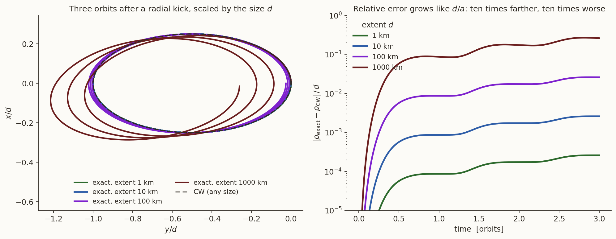
The only approximation was the linearisation of gravity in Section 4.1, and the cost of that approximation is not subtle. We can measure it, by integrating the exact equations of motion of both spacecraft inertially and comparing with the CW prediction for the same initial state. Figure 6 uses a radial kick that produces a CW ellipse of along-track extent \(d\) (so \(A=d/4\)).
For the numbers (codes/cw-verify.py):
| extent \(d\) | \(d/r_t\) | error after \(T\) | after \(3T\) | error\((T)\) / \(d\) |
|---|---|---|---|---|
| \(1\) km | \(1.5\times10^{-4}\) | \(0.087\) m | \(0.26\) m | \(8.7\times10^{-5}\) |
| \(10\) km | \(1.5\times10^{-3}\) | \(8.7\) m | \(26\) m | \(8.7\times10^{-4}\) |
| \(100\) km | \(1.5\times10^{-2}\) | \(0.87\) km | \(2.6\) km | \(8.7\times10^{-3}\) |
| \(1000\) km | \(0.15\) | \(87\) km | \(261\) km | \(8.7\times10^{-2}\) |
The error after one orbit is \(0.59\,d^{2}/r_t\) to within \(0.5\%\) over three decades in \(d\): quadratic in the size of the motion, as the second-order terms of Section 4.1 suggest, and linear in time (compare the \(T\) and \(3T\) columns). The coefficient can be derived exactly, and doing so shows where the error comes from.
Where the error comes from. For this radial kick CW has \(K=\dot y_0+2nx_0=0\) and hence \(\delta a=x_c=0\) (Equation 28): the motion closes forever. The exact chaser is not so lucky. A radial kick \(\Delta v\) is at right angles to the velocity \(v_t\), so the speed becomes \(\sqrt{v_t^{2}+\Delta v^{2}}\) and the specific energy rises by \(\Delta E=\tfrac12\Delta v^{2}\) — a second-order change that the linearisation cannot see. With \(\delta E=\mu\,\delta a/2a^{2}\) and \(\mu=r_tv_t^{2}\),
\[ \delta a=\frac{2r_t^{2}\,\Delta E}{\mu}=r_t\Big(\frac{\Delta v}{v_t}\Big)^{2}, \qquad \Delta v=\frac{nd}{4}\ \Rightarrow\ \frac{\Delta v}{v_t}=\frac{nd}{4\,nr_t}=\frac{d}{4r_t} \]
(the kick \(\Delta v=nd/4\) is what gives a relative ellipse of along-track extent \(d\): its radial semi-axis is \(A=\Delta v/n=d/4\) and its along-track semi-axis \(2A\), Section 6.2).
The chaser is on a slightly higher orbit, so by Kepler’s third law (Section 6.3) its period is longer by \(\Delta T=\tfrac32T\,\delta a/r_t\), and after one target period it lags the target by
\[ v_t\,\Delta T=\tfrac32\,(v_tT)\,\frac{\delta a}{r_t}=\tfrac32\,(2\pi r_t)\,\frac{d^{2}}{16\,r_t^{2}} =\frac{3\pi}{16}\,\frac{d^{2}}{r_t}=0.589\,\frac{d^{2}}{r_t}. \]
This matches the numerical coefficient, \(0.589\), to three figures, and the sign: the exact chaser falls behind CW’s. CW’s error here is a missing second-order change of semi-major axis, and any \(\delta a\) becomes an along-track drift that grows linearly in time.
8.2 Rules of thumb
- The neglected terms are of order \(\rho/r_t\) relative to those kept (Section 4.1). For an orbit-sized relative ellipse of extent \(d\), the position error after one orbit is about \(0.6\,d^{2}/r_t\): about \(9\) m at \(d=10\) km. (The coefficient \(3\pi/16\) is exact for the radial-kick family above; other shapes of relative motion have other coefficients of the same size, but always proportional to \(d^{2}\).)
- Errors accumulate. The neglected terms change the semi-major axis at second order, \(\delta a\sim\rho^{2}/r_t\), and by Kepler’s third law (Section 6.3) any \(\delta a\) is a steady drift. So long propagations degrade, even at short range: the error is linear in the number of orbits.
- Along-track distances are measured along a straight line. The linearisation uses a straight \(y\) axis, whereas the target’s circle curves. A chaser on the same circular orbit, \(100\) km ahead, is at \(x=-s^{2}/2r_t=-0.735\) km, not at \(x=0\); at \(10\) km the offset is \(7\) m. This is a second-order term (\(\eta^{2}\)) and CW does not contain it. Formulations that use curvilinear coordinates remove this particular error (alfriend2010?).
- The target orbit must be circular. For an eccentric target the frame rate is not constant and the coefficients depend on time. The linear relative-motion equations about an elliptic orbit of any eccentricity were obtained by Tschauner and Hempel (tschauner1965?); they reduce to CW as \(e\to0\).
- Only the point-mass force is modelled. Differential drag and the Earth’s oblateness (\(J_2\)) act on the two spacecraft differently and are not in Equation 13; for long propagations they matter more than the second-order gravity terms.
9 Summary
- In the target’s rotating frame (\(\boldsymbol\omega=n\hat{\mathbf k}\)), relative motion obeys the CW equations Equation 13: \(\ddot x-2n\dot y-3n^{2}x=0\), \(\ddot y+2n\dot x=0\) — linear, constant coefficients, coupled through Coriolis. The \(3n^{2}\) is \(2n^{2}\) of tide plus \(n^{2}\) of centrifugal term; the equations are Hill’s, with a target of negligible mass.
- The second equation integrates once: \(\dot y+2nx=K\), the angular-momentum (equivalently energy) difference. With the Jacobi integral it shows that \(x\) oscillates at the orbital frequency about \(x_c=2K/n=4x_0+2\dot y_0/n\).
- The solution is the state transition matrix Equation 24: one matrix multiply propagates a relative state, and \(\mathbf\Phi\) has the group property, the inverse \(\mathbf\Phi(-t)\), and \(\det\mathbf\Phi=1\).
- Every natural motion is a 2:1 epicycle on a drifting guiding centre. The guiding centre sits at \(x_c=\delta a\), the difference of semi-major axes, and drifts at \(-\tfrac32nx_c\): the drift is Kepler’s third law.
- Relative motion is bounded iff \(\dot y_0=-2nx_0\), the condition \(\delta a=0\); otherwise the chaser drifts at \(-3(2nx_0+\dot y_0)\).
- Counter-intuitive but Keplerian: a prograde burn makes you fall behind (\(3T\,\Delta v\) per orbit), a lower orbit drifts ahead, a radial burn closes after one orbit.
- CW is accurate to relative order \(\rho/r_t\): for a radial kick giving a relative ellipse of extent \(d\) the error is exactly the missing second-order \(\delta a\), \(\tfrac{3\pi}{16}d^{2}/r_t\approx0.6\,d^{2}/r_t\) per orbit. Excellent for the last tens of kilometres, which is exactly where the chase deck uses it.
Everything in this note can be reproduced with cw-verify.py: the symbolic checks of the expansions, the solution, the state transition matrix and its eigenstructure, and the numerical examples, including the exact two-body comparisons.
Further reading
For the standard textbook treatments see (curtis2014?) and (vallado2013?); for relative motion in all its forms, with curvilinear coordinates, eccentric targets and \(J_2\), (alfriend2010?).