Time and Ground Tracks
Why every calculation needs a clock, and how to find where a satellite is above the Earth
Where we are going
Every formula we have written so far had a \(t\) in it: Kepler’s equation \(M=n(t-t_0)\), the position of a planet, the angle through which the Earth has turned. We treated \(t\) as a number that somebody else supplies. This note is about the somebody else. It has two unrelated parts.
- Part 1, Time. What is “one day”? Why is a geostationary satellite not in a 24-hour orbit? What are UT1, UTC, TAI, TT and TDB, and why do we need all of them? And, with numerical experiments, why a probe on its way to Mars needs clocks that are good to a few parts in \(10^{12}\) or better.
- Part 2, Ground tracks. How do we turn six orbital elements into the curve that a satellite traces on a map, what does that curve look like for the standard families of orbit (low, polar, sun-synchronous, geosynchronous, Molniya), and what is the curve for? An interactive simulator lets you try any orbit.
The required background is the two-body problem, Kepler’s equation, the orbital elements and the rotation matrices between the perifocal, inertial and Earth-fixed frames. The secular effect of \(J_2\) on \(\Omega\), \(\omega\) and \(M\) is quoted from the note Beyond the Point Mass; nothing else is assumed.
1 Time
1.1 Why time is a first-class variable
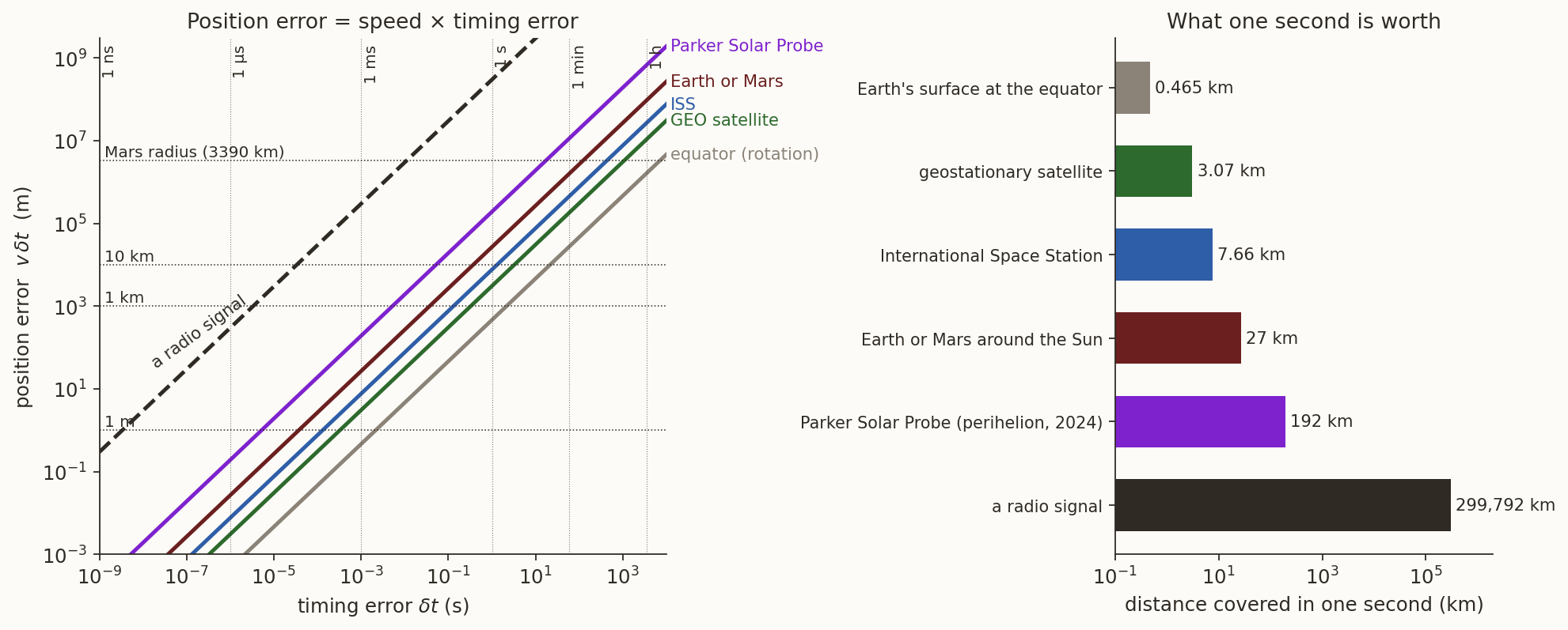
A spacecraft moves, so its position is a function of time, \(\mathbf r(t)\), and a clock that is wrong by \(\delta t\) places it at the wrong point. To first order \[ \delta\mathbf r=\mathbf v\,\delta t,\qquad \delta r = v\,\delta t . \tag{1}\] Figure 1 shows what this means for the objects we deal with. A second is a long time: the International Space Station covers \(7.66\) km in it, the Earth \(29.8\) km along its orbit, and a radio signal \(299\,792\) km. A millisecond is worth \(7.7\) m for the ISS and, for a radio signal, \(300\) km. A nanosecond is \(30\) cm of light travel. Navigation to a metre needs nanoseconds.
History: longitude is time. The Earth turns \(15^\circ\) per hour, so a difference of one hour between local noon and the time on a clock set at a reference meridian means \(15^\circ\) of longitude. In 1714 the British Longitude Act offered £20 000 for a method to find longitude at sea to half a degree, i.e. to two minutes of time, after a voyage of weeks. John Harrison’s fourth chronometer (H4) lost only about five seconds in \(81\) days at sea on its 1761 trial to Jamaica. The problem of the clock is older than the problem of the orbit.
Two questions to keep in mind while reading.
1.2 The day is not one number
1.2.1 Noon to noon and star to star
Two natural clocks are available in the sky: the Sun and the stars. The interval between two successive transits of the Sun across your meridian is the solar day. The interval between two transits of a distant star, which is the time the Earth needs for one complete turn relative to inertial space, is the sidereal day.1 They differ because the Earth moves along its orbit while it turns (Figure 2).
1 Strictly there are two “sidereal” days. The mean sidereal day is measured against the mean equinox of date, which drifts westward against the stars because of precession. The stellar day (the rotation period relative to the International Celestial Reference Frame) is \(8.4\) ms longer. We return to this difference below; for the geometry of this section the two are the same.
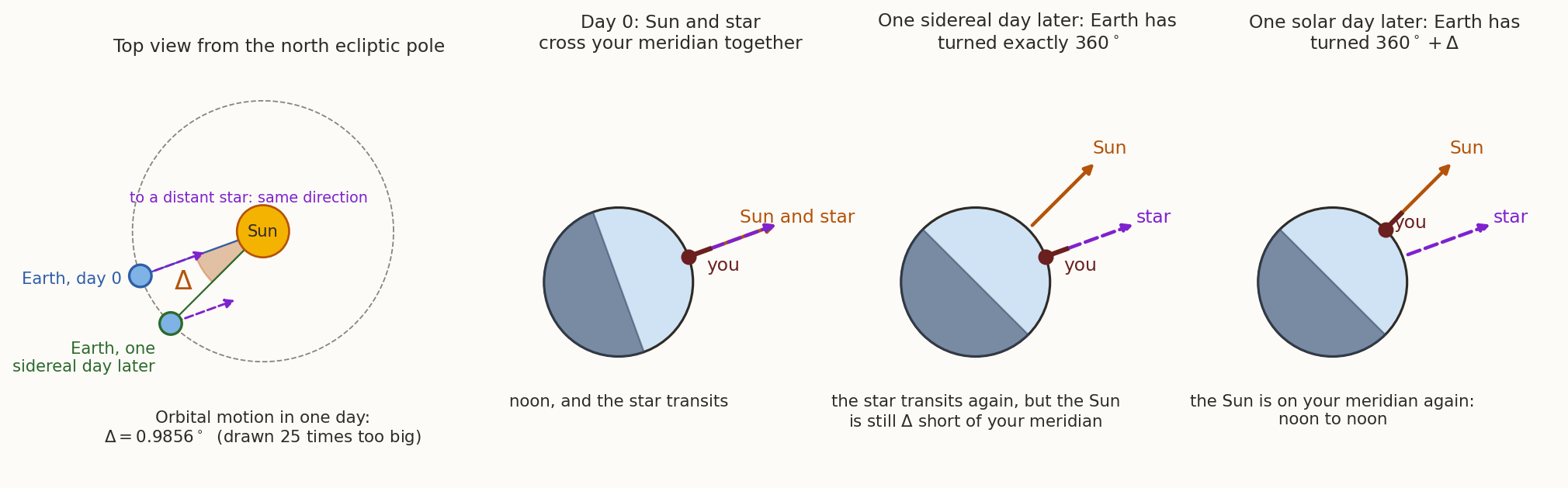
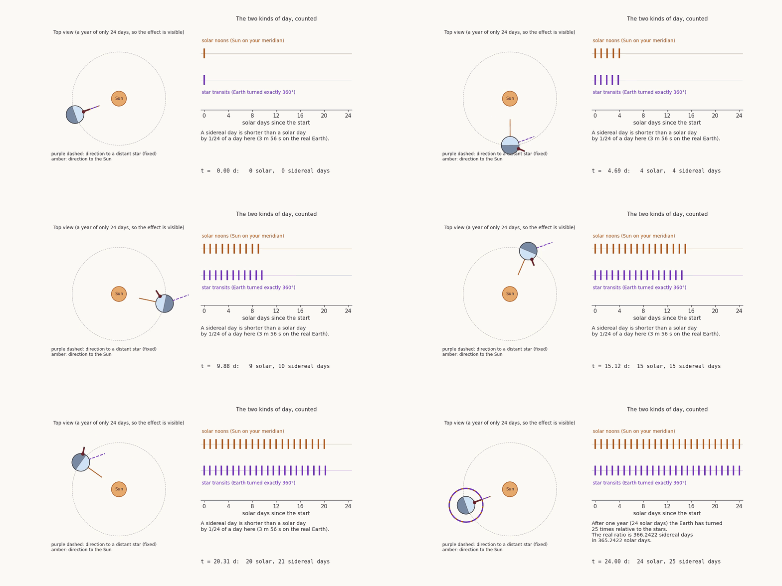
Let \(\omega_\oplus=2\pi/T_{\rm sid}\) be the rotation rate of the Earth relative to the stars and \(n_\odot=2\pi/Y\) the rate at which the Sun’s direction moves as the Earth goes round (the mean motion of the Earth, with \(Y\) the length of the year). The Sun returns to your meridian when the Earth has turned through \(2\pi\) plus the angle the Sun’s direction has moved: \[ \omega_\oplus T_{\rm sol}=2\pi+n_\odot T_{\rm sol} \quad\Longrightarrow\quad \frac{1}{T_{\rm sid}}=\frac{1}{T_{\rm sol}}+\frac{1}{Y}. \tag{2}\] With \(T_{\rm sol}=1\) mean solar day and \(Y=365.242189\) days (the tropical year, the one that defines the seasons), Equation 2 gives \[ T_{\rm sid}=\frac{1}{1+1/365.242189}\ \text{day}=0.99726957\ \text{day}=86\,164.0905\ \text{s}=23\ \text{h}\ 56\ \text{m}\ 4.0905\ \text{s}. \] The Earth therefore has to turn an extra \(\Delta=360^\circ/365.2422=0.9856^\circ\) to bring the Sun back, which takes \(86\,400-86\,164.0905=235.909\) s \(=3\) m \(55.909\) s. Equivalently: one tropical year contains \(365.2422\) solar days but \(366.2422\) sidereal days. The animation below shows this on a planet whose year is only \(24\) days long, so that the extra turn is \(15^\circ\) per day and cannot be missed.
The rotation rate follows directly: \[ \omega_\oplus=\frac{2\pi}{86\,164.0989\ \text{s}}=7.2921151\times10^{-5}\ \text{rad/s}=15.04107^\circ/\text{h}=360.98561^\circ/\text{solar day}, \tag{3}\] where \(86\,164.0989\) s is the stellar day (Table 1). At the equator the surface moves at \(\omega_\oplus R_\oplus=0.4651\) km/s.
| Quantity | Symbol | Value |
|---|---|---|
| Mean solar day (definition, SI seconds) | \(T_{\rm sol}\) | \(86\,400\) s |
| Mean sidereal day (against the mean equinox) | \(T_{\rm sid}\) | \(86\,164.0905\) s \(=23\) h \(56\) m \(4.0905\) s |
| Stellar day (rotation against the ICRF) | \(2\pi/\omega_\oplus\) | \(86\,164.0989\) s |
| Solar day minus sidereal day | \(235.909\) s \(=3\) m \(55.909\) s | |
| Rotation rate against the stars | \(\omega_\oplus\) | \(7.2921151\times10^{-5}\) rad/s |
| Extra turn per day to catch the Sun | \(\Delta\) | \(0.9856^\circ\) |
1.2.2 What the difference does to spaceflight
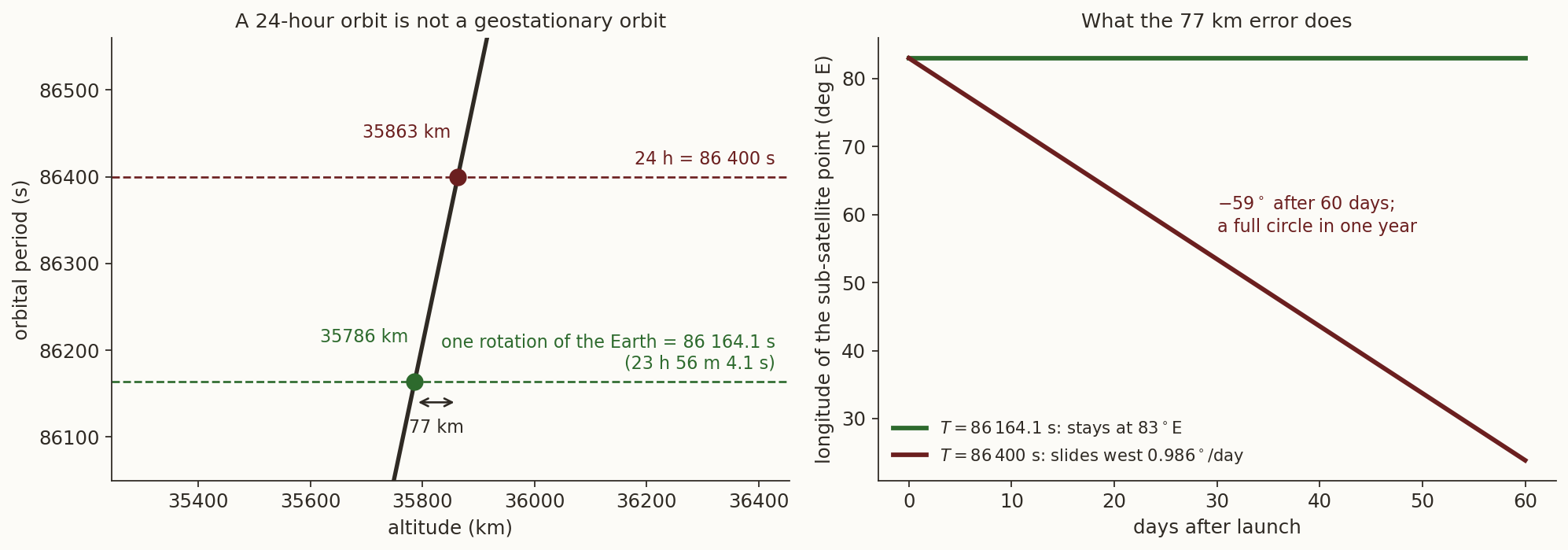
Geostationary orbit. A satellite stays above one point of the equator only if it goes round in the time the Earth takes to turn once relative to inertial space, which is the sidereal (stellar) day and not \(24\) h. Kepler’s third law \(a^3=\mu\,(T/2\pi)^2\) gives \[ T=86\,164.0989\ \text{s}\ \Rightarrow\ a=42\,164.17\ \text{km},\ h=35\,786.03\ \text{km};\qquad T=86\,400\ \text{s}\ \Rightarrow\ a=42\,241.10\ \text{km},\ h=35\,862.96\ \text{km}. \] The two orbits differ by only \(76.9\) km in radius. A satellite placed in the \(24\)-hour orbit turns through \(360^\circ\) per \(86\,400\) s while the Earth turns through \(360.9856^\circ\): it falls behind by \(0.9856^\circ\) per day, drifting west at the rate at which the Sun moves along the ecliptic. After \(60\) days it is \(59^\circ\) from where it started, and after a year it has been all the way round (Figure 4). One degree of longitude on the geostationary ring is \(736\) km.
Launch windows. To launch into a given orbital plane, the launch site must pass through that plane, and the plane is fixed in inertial space (to zeroth order). The site returns to the same inertial direction once per sidereal day, so an instantaneous launch window opens \(3\) m \(56\) s earlier each day. If the plane itself turns, as the orbit of the International Space Station does at \(\dot\Omega=-4.95^\circ\)/day because of \(J_2\), the Earth must turn through \(360^\circ+4.95^\circ\) relative to the plane and the windows recur every \(2\pi/(\omega_\oplus-\dot\Omega)=23.61\) h, about \(24\) minutes earlier each day.
Sun-synchronous orbits. The condition for an orbit to keep a fixed angle to the Sun is that its plane turns at \(0.9856^\circ\)/day, the rate at which the Sun’s direction moves in Figure 2 (see Section 2.3.3). For such an orbit the Earth turns through exactly \(360^\circ\) relative to the plane in one mean solar day, which is why repeat cycles of Earth-observation satellites are quoted in solar days.
Frames. The rotation between the inertial (ECI) and Earth-fixed (ECEF) frames is a rotation about the polar axis through the Greenwich sidereal angle. This is the only place where the Earth’s rotation, and thus this section, enters a ground-track or ground-station calculation (Section 2.2).
1.2.3 The solar day is not even constant
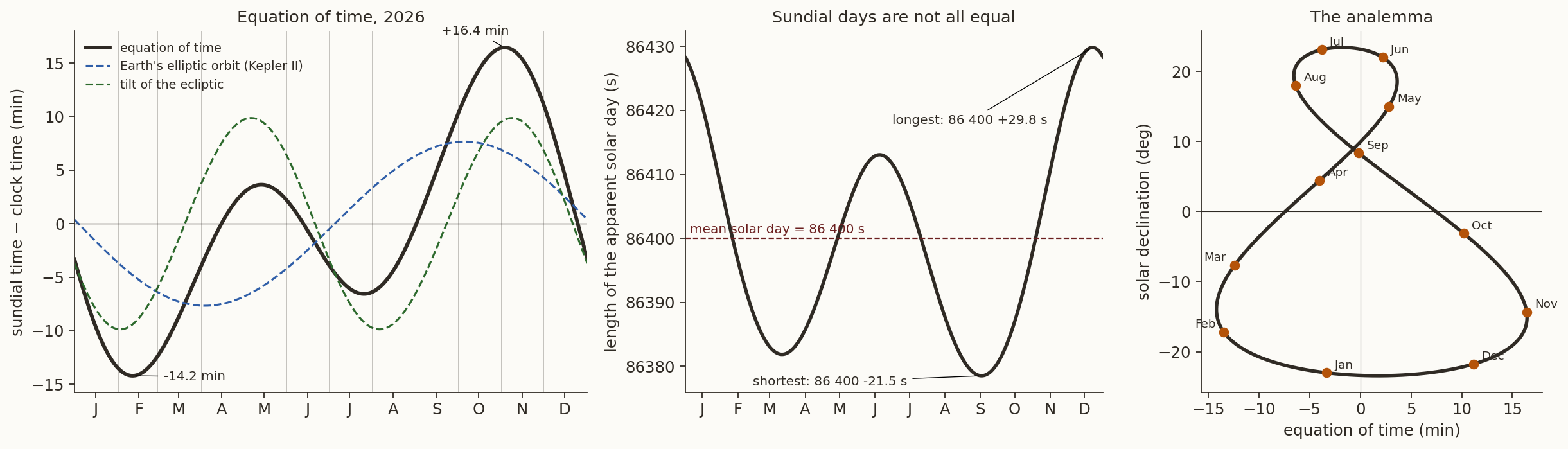
So far we have used the mean solar day. A sundial does not keep mean time. Two effects make the real Sun’s hour angle advance non-uniformly: the Earth moves faster near perihelion (Kepler’s second law), and the Sun moves along the ecliptic, which is inclined \(23.44^\circ\) to the equator, while hour angle is measured along the equator. The equation of time is the difference between sundial time and the time of a uniform “mean sun”, \[ {\rm EoT}=L-\alpha , \tag{4}\] where \(L\) is the mean longitude of the Sun (uniform in time) and \(\alpha\) its true right ascension. The first cause contributes \(-(\text{equation of centre})\), of amplitude \(7.7\) min; the second, \(\lambda-\alpha\approx\tan^2(\epsilon/2)\sin2\lambda\), of amplitude \(9.9\) min. The sum reaches \(+16.4\) min in early November and \(-14.2\) min in mid-February (Figure 5).
Because EoT changes with time, sundial days are not all \(86\,400\) s long. An apparent solar day equals \(86\,400\) s minus the rate of change of EoT; near December \(22\) it lasts \(86\,400+29.9\) s, near September \(16\) it lasts \(86\,400-21.5\) s. The mean over the year is \(86\,400\) s by construction. This is the reason the civil second is tied to a mean sun, and the reason sidereal time, which has no such variation, is the natural angle for frame rotations.
1.2.4 Years and months
The same reasoning applies to the year. Which year we mean depends on what we compare the Earth’s position with.
| Year | Compared with | Length (days) |
|---|---|---|
| Tropical | the equinox (seasons); shortened by precession | \(365.242189\) |
| Sidereal | the fixed stars: one true revolution | \(365.256363\) |
| Anomalistic | the perihelion (apsides advance \(11.6''\)/yr) | \(365.259636\) |
The Moon obeys Equation 2 too, with the sidereal month \(27.321662\) d in place of \(T_{\rm sid}\) and the year for \(Y\): \[ \frac{1}{T_{\rm syn}}=\frac{1}{27.321662}-\frac{1}{365.256363}\quad\Rightarrow\quad T_{\rm syn}=29.530589\ \text{d}, \] the synodic month, from new moon to new moon. A lunar lander’s sunlit period is set by the synodic month, not the sidereal one: this is why the lunar day is about \(14\) Earth days of sunlight, and why the Chandrayaan-3 landing was timed for lunar dawn at the landing site.
1.3 Time scales
1.3.1 Three families
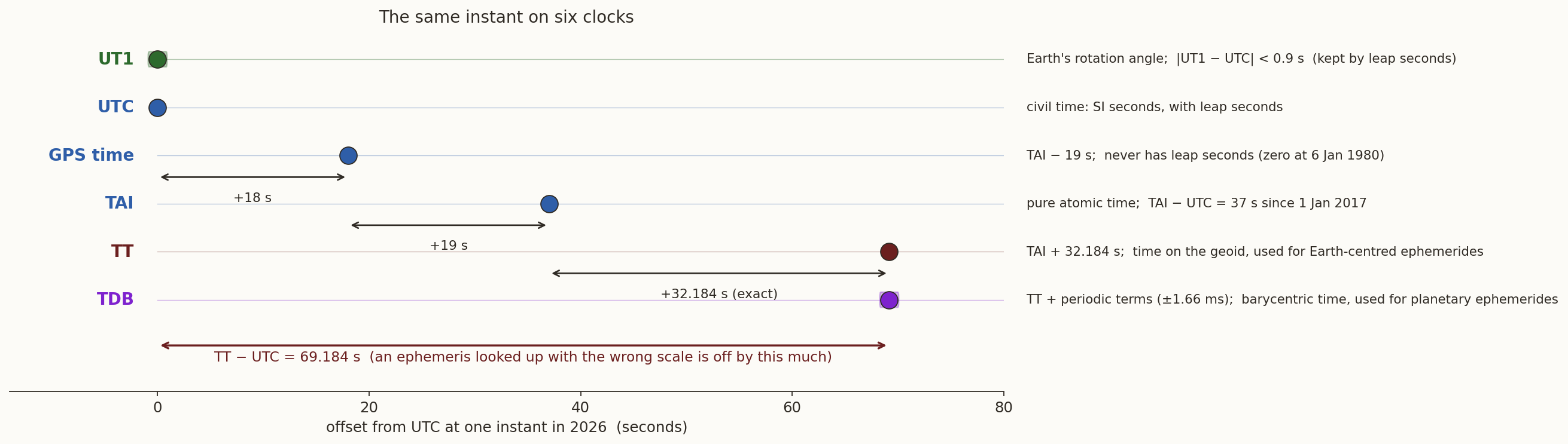
A “time” is an agreement about what a second is and where the zero is. Three families are in use in space flight (Figure 6 and Table 3).
- Rotational time, UT1. Defined by the rotation angle of the Earth; it is what the transformation ECI \(\leftrightarrow\) ECEF needs. It is irregular, because the Earth’s rotation is.
- Atomic time, TAI, UTC, GPS time. Defined by the SI second: \(9\,192\,631\,770\) periods of the hyperfine transition of caesium-133. TAI counts these seconds continuously. UTC, the civil time, uses the same seconds but is inserted with occasional leap seconds so that it stays within \(0.9\) s of UT1. GPS time is TAI shifted by a constant.
- Dynamical time, TT and TDB. The independent variable of the equations of motion. TT (Terrestrial Time) is the time on the geoid, an ideal continuation of TAI: TT \(=\) TAI \(+\,32.184\) s. TDB (Barycentric Dynamical Time) is the time for equations of motion about the solar-system barycentre; it differs from TT by periodic terms of up to \(1.66\) ms (Section 1.3.3). Planetary ephemerides are functions of TDB.
| Scale | Definition | Offset from UTC now | Used for |
|---|---|---|---|
| UT1 | Earth rotation angle | \(\mathrm{UT1-UTC}=\pm0.9\) s at most | ECI \(\leftrightarrow\) ECEF; sidereal time |
| UTC | atomic seconds with leap seconds | \(0\) | civil time; tracking-station clocks |
| GPS time | \(\text{TAI}-19\) s | \(+18\) s | GNSS receivers and products |
| TAI | atomic seconds, continuous | \(+37\) s | the basis of the atomic scales |
| TT | \(\text{TAI}+32.184\) s | \(+69.184\) s | Earth-centred ephemerides, precession |
| TDB | \(\text{TT}+\) periodic terms | \(+69.184\) s \(\pm1.7\) ms | planetary ephemerides |
History: from the Earth to the atom. Until 1956 the second was \(1/86\,400\) of the mean solar day. Louis Essen and Jack Parry built the first caesium clock at the National Physical Laboratory in 1955 and showed that it was far steadier than the Earth. The SI second was redefined by caesium in 1967. UTC in its present form started on 1 January 1972 with \(10\) s already added; \(27\) leap seconds followed, the last on 31 December 2016. In 2022 the General Conference on Weights and Measures resolved to stop inserting leap seconds by 2035, letting UT1 \(-\) UTC grow beyond \(0.9\) s.
The epoch used everywhere in modern ephemerides is J2000.0: 2000 January 1, 12:00 TT, which is Julian date \(2\,451\,545.0\). Time in Julian centuries is \(T=(\mathrm{JD}-2\,451\,545.0)/36\,525\).
1.3.2 The Earth as a clock
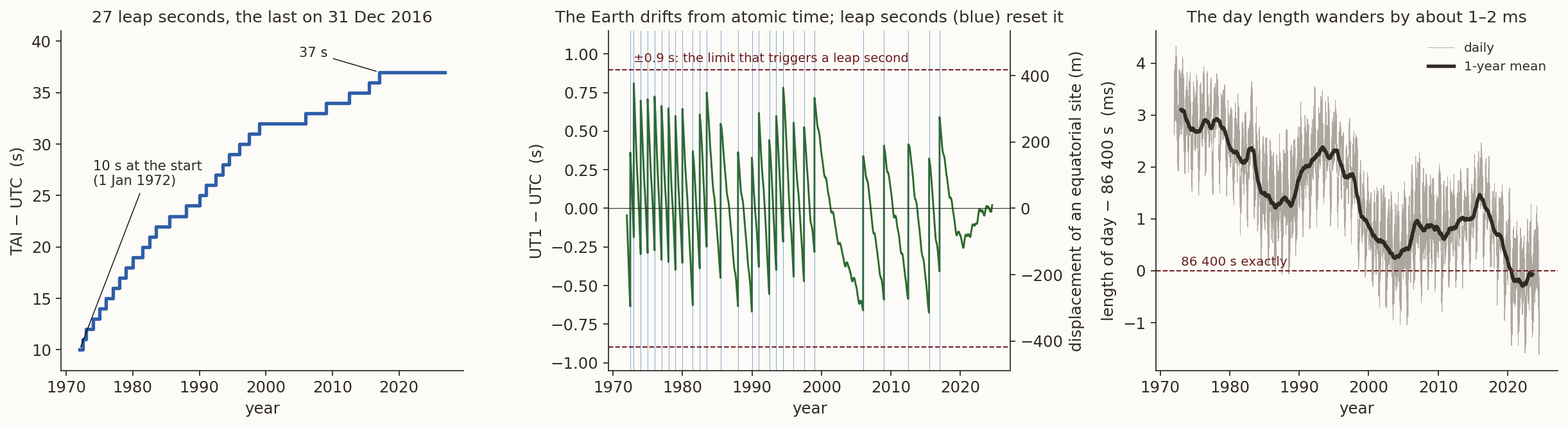
Figure 7 shows what forces us to keep two kinds of time. The left panel is the staircase of leap seconds. The middle panel is \(\mathrm{UT1}-\mathrm{UTC}\), from the IERS Earth-orientation series: since \(1972\) the Earth’s rotation has usually run slow against the atomic clocks, so \(\mathrm{UT1}-\mathrm{UTC}\) drifts downward and a leap second resets it. The right panel is the excess length of day (LOD), the difference between the true rotation period and \(86\,400\) s, obtained as \(-\,\mathrm d(\mathrm{UT1}-\mathrm{TAI})/\mathrm dt\).
The rotation of the Earth changes for many reasons: tidal friction with the Moon lengthens the day by about \(2\) ms per century over the long term; exchanges of angular momentum with the atmosphere and oceans (seasonal, El Niño) and with the liquid core (decades) move it around by a millisecond or more. In these data the day was about \(3\) ms longer than \(86\,400\) s in the \(1970\)s, and since about \(2020\) the Earth has been spinning faster: the shortest day in the series, \(1.62\) ms short, is \(5\) July 2024. Nobody can predict these changes beyond a few weeks, which is why UT1 \(-\) UTC must be measured (by very-long-baseline interferometry and satellite laser ranging) and published by the IERS.
The practical consequence for us: if you build the ECI-to-ECEF rotation from UTC instead of UT1 you make a rotation error of up to \(0.9\) s \(\times\,15.04''\)/s \(=13.5''\), which moves a point on the equator by \(\omega_\oplus R_\oplus\times0.9\ \text{s}=419\) m (right axis of the middle panel).
1.3.3 Relativity: TDB against TT
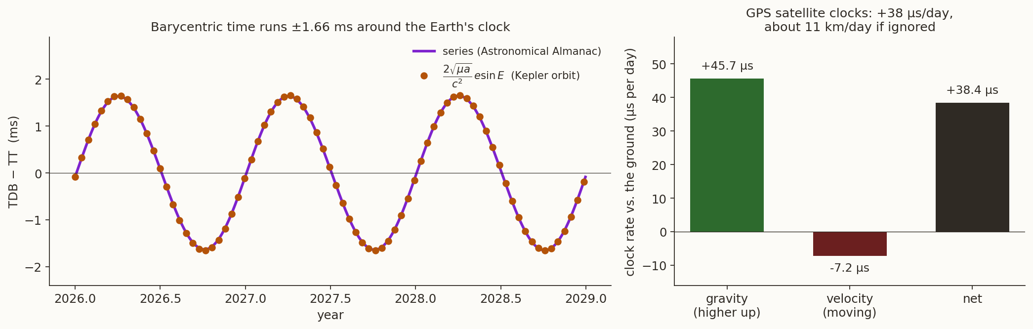
Why do TT and TDB differ at all? A clock at rest on the geoid and a clock at rest at the solar-system barycentre tick at different rates, because they sit at different gravitational potentials and move at different speeds. To first order in \(1/c^2\) a clock at distance \(r\) from the Sun, moving with speed \(v\), runs at \[ \frac{d\tau}{dt}=1-\frac{1}{c^{2}}\left(\frac{v^2}{2}+\frac{\mu_\odot}{r}\right). \tag{5}\] For a Keplerian orbit of the Earth, \(v^2=\mu_\odot(2/r-1/a)\), so the bracket is \(2\mu_\odot/r-\mu_\odot/2a\). Integrate over time using \(r=a(1-e\cos E)\) and \(n\,dt=(1-e\cos E)\,dE\), which gives \(\int dt/r=E/(na)\) and \(\mu_\odot/(na)=\sqrt{\mu_\odot a}\). Then with Kepler’s equation \(E=nt+e\sin E\), \[ \tau-t=\underbrace{\left(\frac{\mu_\odot}{2ac^2}-\frac{2\sqrt{\mu_\odot a}\,n}{c^2}\right)t}_{\text{a constant rate, absorbed into the definition of TT}}\;-\;\frac{2\sqrt{\mu_\odot a}}{c^{2}}\,e\sin E . \tag{6}\] The linear term only says that the two clocks were defined with slightly different rates. What is left is a periodic term: TDB \(-\) TT \(=+\dfrac{2\sqrt{\mu_\odot a}}{c^2}\,e\sin E\), whose amplitude for the Earth (\(a=1\) AU, \(e=0.016709\)) is \(1.6568\) ms. The Astronomical Almanac series, which includes the effect of the other planets, has amplitude \(1.657\) ms and follows Equation 6 to within \(24\) µs (Figure 8, left). Physically, the Earth is faster and deeper in the Sun’s potential at perihelion (early January), so its clock runs slow relative to the barycentre then.
The same Equation 5 applies to a satellite around the Earth. For a GPS satellite (\(a=26\,560\) km) relative to a clock on the geoid, \[ \frac{\Delta\tau}{\tau}=\frac{\mu_\oplus}{c^2}\left(\frac{1}{R_\oplus}-\frac1a\right)-\frac{\mu_\oplus}{2ac^2}=+5.28\times10^{-10}-0.83\times10^{-10}=+4.45\times10^{-10}, \] i.e. the satellite clock runs fast by \(+45.7\ \mu\)s per day because it is higher in the potential and slow by \(7.2\ \mu\)s per day because it moves; the net is \(+38.4\ \mu\)s per day. Multiplied by \(c\), \(38.4\ \mu\text{s}\) is \(11.5\) km of ranging error per day if it were not corrected. The correction is built into the satellite oscillator frequency before launch (the clock is deliberately tuned slightly slow on the ground).
1.3.4 Julian date and sidereal time in practice
The course text (Curtis) gives working formulas, valid for \(1901\) to \(2099\). The Julian date at \(0\) h UT of calendar date \((y,m,d)\) is \[ J_0=367\,y-\operatorname{INT}\!\left\{\frac{7\left[y+\operatorname{INT}\!\left(\frac{m+9}{12}\right)\right]}{4}\right\}+\operatorname{INT}\!\left(\frac{275\,m}{9}\right)+d+1\,721\,013.5,\qquad \mathrm{JD}=J_0+\frac{\mathrm{UT}}{24}, \tag{7}\] with UT in hours. The Greenwich sidereal time at \(0\) h UT follows from \(T_0=(J_0-2\,451\,545)/36\,525\), \[ \theta_{G0}=100.4606184^\circ+36\,000.77004^\circ\,T_0+0.000387933^\circ\,T_0^{2}-2.583\times10^{-8}\,T_0^{3}, \tag{8}\] and at a later universal time UT (hours), \[ \theta_G=\theta_{G0}+360.98564724^\circ\,\frac{\mathrm{UT}}{24}. \tag{9}\] The coefficient \(360.98564724\) is \(360^\circ\) times the number of sidereal days in a solar day, \(1.00273790935\), and is the rate of Equation 3 measured against the equinox. The local sidereal time at east longitude \(\lambda_E\) is \(\theta_G+\lambda_E\); it equals the right ascension of the stars on your meridian. In code:
def julian_date(y, m, d, ut_hours=0.0):                     # Curtis (5.48)
    j0 = 367*y - int(7*(y + int((m + 9)/12))/4) + int(275*m/9) + d + 1721013.5
    return j0 + ut_hours/24

def gmst_deg(y, m, d, ut_hours):                            # Curtis (5.49)-(5.50), degrees
    t0 = (julian_date(y, m, d) - 2451545)/36525
    th0 = 100.4606184 + 36000.77004*t0 + 0.000387933*t0**2 - 2.583e-8*t0**3
    return (th0 + 360.98564724*ut_hours/24) % 360
For example, \(J_0\) for 2026 September 29 is \(2\,461\,312.5\), so noon UT that day is JD \(2\,461\,313.0\). The sidereal-time formulas agree with astropy’s IAU 1982 model to about \(10^{-4}\) degrees once UT1 (not UTC) is used for the argument, and our leap-second table agrees with the ERFA table at more than a hundred dates between \(1972\) and \(2026\). The code is in _timeutil.py.
1.4 What a clock error costs: numerical experiments
We now put numbers on the question in the title of Part 1. All experiments use the planetary positions of a real ephemeris (the built-in one of astropy, good to arcseconds, ample for this purpose).
1.4.1 Two ways a clock enters navigation
Time tags. Every state, every ephemeris lookup, every command is stamped with an epoch. If the stamp is wrong by \(\delta t\), Equation 1 applies directly.
Measurements. Deep-space navigation is done with radio signals, and each measurement is a comparison with a clock. A two-way range measures the round-trip time \(\tau\) of a signal transmitted at \(t_t\) and received at \(t_r\) by the same ground clock: \[ \rho=\tfrac12\,c\,(t_r-t_t)=\tfrac12 c\tau . \tag{10}\] A Doppler measurement compares the frequency of the received carrier with that of the transmitted one, and gives the range rate \(\dot\rho=-\tfrac12\,c\,\Delta f/f\) for a two-way link (\(\dot\rho=-c\,\Delta f/f\) one-way). Therefore range is a time measurement and range rate is a frequency measurement: an error of one nanosecond in \(\tau\) is \(15\) cm of range; a fractional error \(\varepsilon\) in the frequency reference is a velocity error \(c\,\varepsilon\).
1.4.2 Experiment 1: how far is Mars, in minutes?
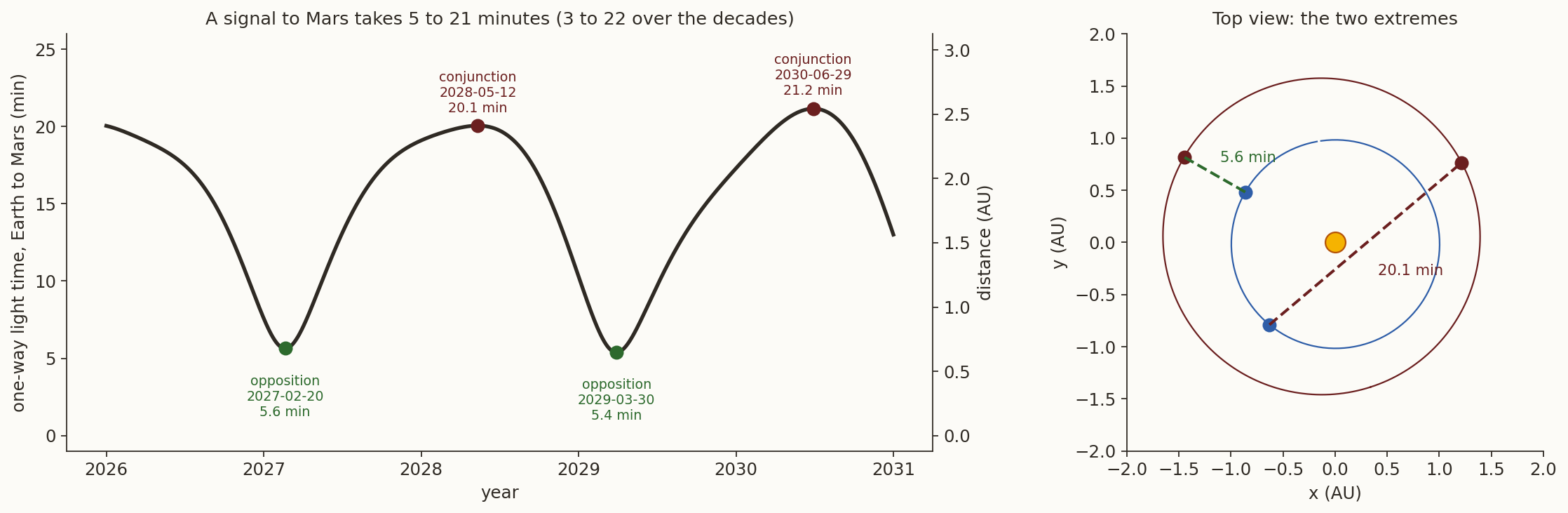
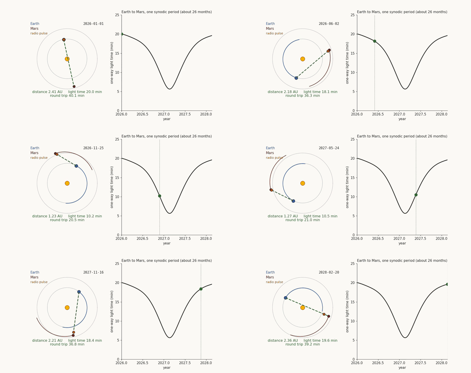
The first thing a clock has to do at planetary distances is to bridge the light time. Figure 9 shows the one-way light time between Earth and Mars for the next five years, and the animation shows the geometry behind it. The light time varies between \(5.4\) min at the oppositions of \(2027\) and \(2029\) (\(0.68\) and \(0.65\) AU) and \(21.2\) min at the conjunction of June \(2030\) (\(2.55\) AU). Over several decades the extremes are \(3.1\) and \(22.3\) min (\(0.37\) and \(2.68\) AU).
Consequences: there is no possibility of “flying” a spacecraft from Earth. A command is executed at a time on the spacecraft clock that was chosen at least one light time earlier, so the ground must know the relation between the spacecraft clock and UTC to far better than the accuracy demanded of the event. When India’s Mars Orbiter Mission was inserted into orbit on 24 September 2014 the distance was \(1.499\) AU (\(224\) million km), the one-way light time \(12.5\) min and the round trip \(24.9\) min; the whole braking sequence had to be uploaded in advance.
1.4.3 Experiment 2: a clock that is slightly wrong
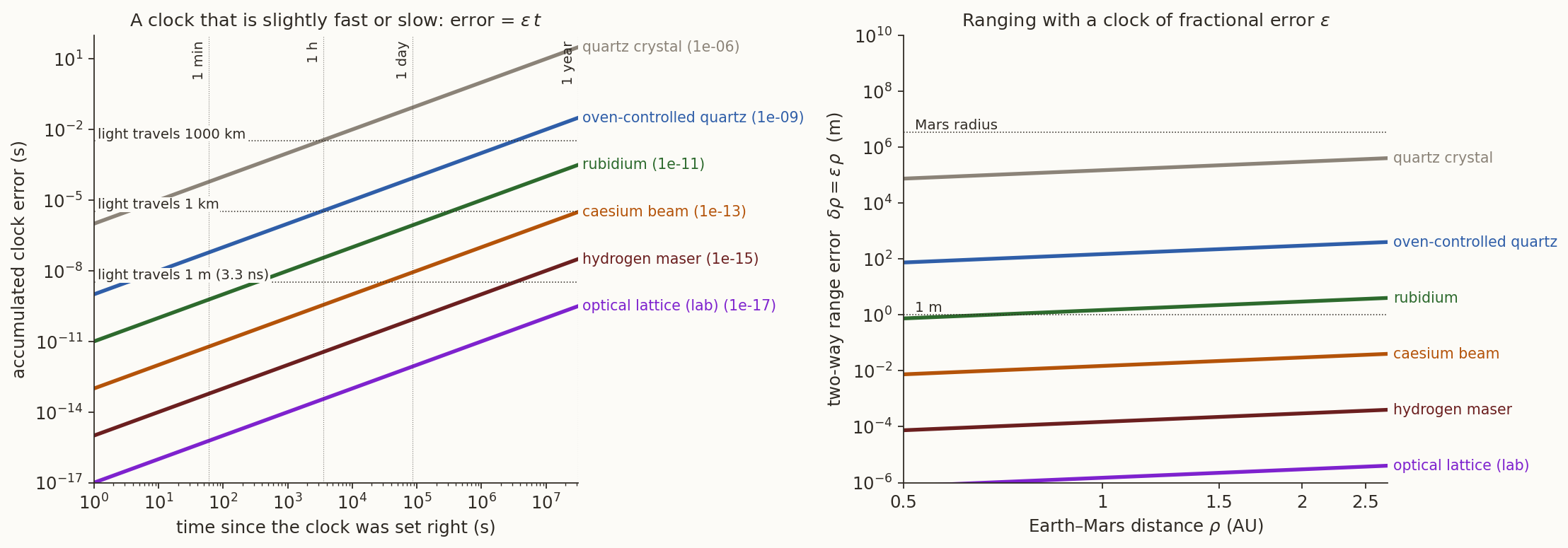
Suppose a ground clock runs fast or slow by the fractional amount \(\varepsilon\). After a time \(t\) it is wrong by \(\varepsilon t\) (Figure 11, left), and a ranging measurement that spans a round trip \(\tau=2\rho/c\) is wrong by \(\varepsilon\tau\), i.e. the range error is \[ \delta\rho=\varepsilon\,\rho . \tag{11}\] It is the fractional error of the clock that matters, and it multiplies the whole distance (Figure 11, right). Table 4 lists representative values for oscillator classes (orders of magnitude of an uncalibrated frequency offset, not datasheet values).
| Oscillator | \(\varepsilon\) | Time error after \(1\) day | \(\delta\rho\) at \(1.5\) AU |
|---|---|---|---|
| quartz crystal | \(10^{-6}\) | \(86\) ms | \(224\) km |
| oven-controlled quartz | \(10^{-9}\) | \(86\) µs | \(224\) m |
| rubidium | \(10^{-11}\) | \(0.86\) µs | \(2.2\) m |
| caesium beam | \(10^{-13}\) | \(8.6\) ns | \(2.2\) cm |
| hydrogen maser | \(10^{-15}\) | \(0.09\) ns | \(0.22\) mm |
| optical lattice (laboratory) | \(10^{-17}\) | \(0.9\) ps | \(2\) µm |
To range to \(1\) m the round-trip time must be timed to \(2\rho/c\) within \(6.7\) ns, and over the light time of Mars the clock must be better than \(\varepsilon=4.5\times10^{-12}\) at \(1.5\) AU and \(2.7\times10^{-12}\) at \(2.5\) AU. A rubidium clock is marginal; a caesium clock or a hydrogen maser is comfortable. A quartz oscillator is hopeless: at \(1.5\) AU it would place Mars \(224\) km away from where it is.
1.4.4 Experiment 3: from a frequency error to a miss distance
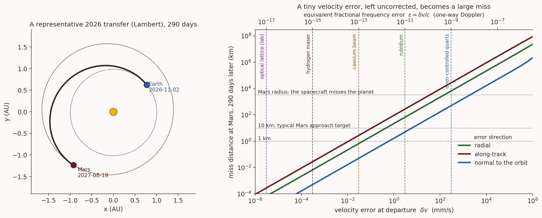
Doppler is even more demanding, because a velocity error grows into a position error over the whole flight. We compute this for a representative \(2026\) Earth–Mars transfer: depart on \(2\) November \(2026\), arrive on \(19\) August \(2027\), \(290\) days later. The planets’ heliocentric positions come from the ephemeris and the transfer conic is found with Lambert’s method (universal variables). The result is a departure \(v_\infty=3.03\) km/s (\(C_3=9.2\) km\(^2\)/s\(^2\)) and an arrival \(v_\infty=2.73\) km/s, from \(0.99\) AU to \(1.54\) AU (Figure 12, left).
Now perturb the heliocentric velocity at departure by \(\delta v\) in three directions (radial, along-track, normal to the orbit), propagate the two-body orbit for \(290\) days, and measure the distance from Mars at the nominal arrival time. The state-transition matrix from departure velocity to arrival position has singular values of \(94.1\), \(10.5\) and \(1.7\) km per mm/s. In numbers:
| Velocity error at departure | radial | along-track | normal |
|---|---|---|---|
| \(1\) mm/s | \(22\) km | \(92\) km | \(1.7\) km |
| \(1\) cm/s | \(221\) km | \(921\) km | \(17\) km |
| \(1\) m/s | \(22\,100\) km | \(92\,100\) km | \(1\,680\) km |
A velocity error of \(1\) mm/s costs \(92\) km at Mars, and a target of \(10\) km (typical for the approach to a planet) needs the velocity known to \(0.1\) mm/s. The connection with clocks is Equation 1 in the frequency domain: a fractional frequency error \(\varepsilon\) in a one-way Doppler link is a velocity error \(c\varepsilon\), so the top axis of Figure 12 (right) is the same as the bottom one divided by \(c\). For the worst direction, \(10\) km at Mars requires \(\varepsilon\lesssim3.5\times10^{-13}\): an oven-controlled quartz oscillator (\(10^{-9}\), \(0.3\) m/s) would miss Mars by \(28\,000\) km, a rubidium clock (\(10^{-11}\), \(3\) mm/s) by \(280\) km, a caesium clock (\(10^{-13}\), \(0.03\) mm/s) by \(2.8\) km and a hydrogen maser (\(10^{-15}\)) by \(28\) m.
1.4.5 Experiment 4: the ledger of wrong time scales
The most common time mistakes are not physical: they are bookkeeping errors, a wrong scale or a forgotten offset. Their cost follows from Equation 1 with the true speeds (Earth \(29.4\) km/s and Mars \(23.8\) km/s at the arrival date; \(7.61\) km/s for a \(500\) km orbit). We checked the first two rows by shifting the ephemeris epoch.
| Mistake | \(\delta t\) | Consequence |
|---|---|---|
| Look up planetary positions with UTC where TDB (or TT) is required | \(69.184\) s | Mars is \(1\,648\) km from its true position, the Earth \(2\,035\) km |
| Ignore a single leap second | \(1\) s | Earth \(29\) km, Mars \(24\) km |
| Use UTC where TAI is required (after 2017) | \(37\) s | Earth \(1\,088\) km, Mars \(882\) km |
| Treat GPS time as UTC | \(18\) s | a \(500\) km satellite is \(137\) km off along its track |
| Use UTC for UT1 in the ECI \(\to\) ECEF rotation | \(\le0.9\) s | up to \(419\) m on the ground at the equator |
| Ignore TDB \(-\) TT | \(1.66\) ms | Earth \(49\) m, Mars \(40\) m |
| Ranging to \(1\) m | \(6.7\) ns | a clock error of \(10\) ns is \(3\) m |
Part 1 in one paragraph. Position error is speed times time error (Equation 1); range is a time measurement and Doppler a frequency measurement. A day is \(86\,400\) s of solar time but \(86\,164.09\) s for one turn of the Earth, and the difference (\(3\) m \(56\) s) explains the geostationary altitude, launch windows and sun-synchronous orbits. Time comes in three families: UT1 (rotation), atomic (TAI, UTC, GPS) and dynamical (TT, TDB); today TAI \(-\) UTC \(=37\) s, TT \(-\) UTC \(=69.184\) s and TDB differs from TT by \(\pm1.66\) ms, which follows from Equation 5. For a Mars mission range needs nanoseconds and velocity needs fractional frequency stability of order \(10^{-13}\) or better, which is hydrogen-maser territory.
2 Ground tracks
2.1 What is a ground track?
The ground track of a satellite is the curve that the sub-satellite point traces on the surface of the Earth as the Earth turns beneath the orbit. The sub-satellite point is the point where the line from the satellite to the Earth’s centre (or, more precisely, the local vertical) pierces the surface. It is described by a latitude \(\varphi\) and an east longitude \(\lambda\).
The ground track answers the questions “what does the satellite see?”, “when is it over my station?” and “when will it return to the same place?”. Almost every application (Section 2.5) is a statement about the ground track.
2.2 The method, step by step
The orbit is a fixed ellipse in inertial space. The ground track appears because the Earth turns beneath it. That is the whole idea, and it separates the computation into two parts: find the position in an inertial frame (steps 2 to 4 of Figure 13), then express it in the Earth-fixed frame (steps 5 and 6).
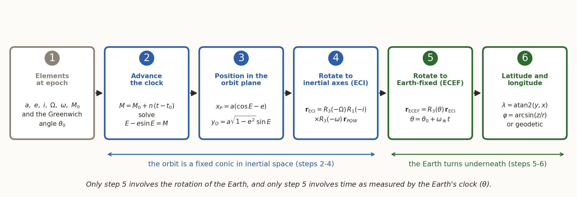
Step 1: the data. The six elements \((a,e,i,\Omega,\omega,M_0)\) at the epoch \(t_0\), and the Greenwich sidereal angle \(\theta_0\) at the epoch, from Equation 9.
Step 2: advance the clock. With \(t\) the time since the epoch, the mean anomaly is \(M=M_0+n(t-t_0)\), \(n=\sqrt{\mu/a^3}\), and Kepler’s equation \(E-e\sin E=M\) is solved for \(E\) (Newton’s method).
Step 3: position in the orbit plane (perifocal frame, \(\hat{\mathbf p}\) towards perigee): \[ x_P=a(\cos E-e),\qquad y_Q=a\sqrt{1-e^{2}}\,\sin E,\qquad z_W=0 . \tag{12}\]
Step 4: to inertial axes. Three rotations bring the orbit plane to its place: about the normal by \(\omega\) (perigee direction), about the line of nodes by \(i\) (tilt), about the polar axis by \(\Omega\) (node). With \(R_1\) and \(R_3\) the passive rotation matrices about \(x\) and \(z\), \[ \mathbf r_{\rm ECI}=R_3(-\Omega)\,R_1(-i)\,R_3(-\omega)\,\mathbf r_{PQW},\qquad R_3(\theta)=\begin{pmatrix}\cos\theta&\sin\theta&0\\-\sin\theta&\cos\theta&0\\0&0&1\end{pmatrix},\quad R_1(\theta)=\begin{pmatrix}1&0&0\\0&\cos\theta&\sin\theta\\0&-\sin\theta&\cos\theta\end{pmatrix}. \tag{13}\]
Step 5: to Earth-fixed axes. The Earth-fixed frame is the inertial frame turned about the polar axis through the Greenwich angle \(\theta(t)=\theta_0+\omega_\oplus(t-t_0)\), with \(\omega_\oplus\) from Equation 3: \[ \mathbf r_{\rm ECEF}=R_3\bigl(\theta(t)\bigr)\,\mathbf r_{\rm ECI}. \tag{14}\]
Step 6: latitude and longitude. With \((x,y,z)=\mathbf r_{\rm ECEF}\) and \(r=|\mathbf r|\), the geocentric coordinates are \[ \lambda=\operatorname{atan2}(y,x),\qquad \varphi_{\rm gc}=\arcsin\frac zr . \tag{15}\] Maps and GPS use the geodetic latitude, measured from the local normal to the WGS-84 ellipsoid (flattening \(f=1/298.257\)). It is obtained by a short iteration (Bowring), with \(p=\sqrt{x^2+y^2}\), \(e_E^2=f(2-f)\): \[ \varphi\leftarrow\operatorname{atan2}\!\left(z,\;p\Bigl(1-e_E^{2}\tfrac{N}{N+h}\Bigr)\right),\quad N=\frac{R_\oplus}{\sqrt{1-e_E^{2}\sin^{2}\varphi}},\quad h=\frac{p}{\cos\varphi}-N , \tag{16}\] started from \(\varphi=\operatorname{atan2}(z,\,p(1-e_E^2))\); six passes converge to well below a millimetre. The geodetic and geocentric latitudes differ by at most \(0.19^\circ\) (about \(21\) km on the ground), so for a picture at the scale of a continent either will do, but for pointing an antenna it matters.
def ground_track(a, e, i, raan, argp, M0, t, theta0=0.0):
    n = np.sqrt(mu/a**3)
    E = kepler(M0 + n*t, e)
    xp, yq = a*(np.cos(E) - e), a*np.sqrt(1 - e*e)*np.sin(E)             # (3)
    r_eci = R3(-raan) @ R1(-i) @ R3(-argp) @ np.array([xp, yq, 0])       # (4)
    r_ecef = R3(theta0 + omega_E*t) @ r_eci                               # (5)
    return np.degrees(np.arctan2(r_ecef[1], r_ecef[0])), \
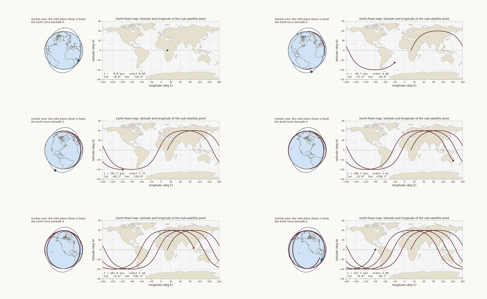
np.degrees(np.arcsin(r_ecef[2]/np.linalg.norm(r_ecef))) # (6)The animation shows the two views together for an orbit of \(60^\circ\) inclination and \(1200\) km altitude. On the left, the orbit plane (blue ring) does not move; the globe turns beneath it, and the red curve is painted on the rotating surface. On the right is the same curve on a map.
2.2.1 A closed form for circular orbits
For a circular orbit (\(e=0\)) the six steps collapse into a formula that we can read. Use the argument of latitude \(u=\omega+f\) (the angle from the ascending node to the satellite, measured in the orbit plane). Steps 3 and 4 give the inertial unit vector \[ \hat{\mathbf r}_{\rm ECI}=\bigl(\cos\Omega\cos u-\sin\Omega\cos i\sin u,\ \ \sin\Omega\cos u+\cos\Omega\cos i\sin u,\ \ \sin i\sin u\bigr). \] The last component is \(\sin\varphi\) directly, and the first two can be combined as \(x+\mathrm iy=e^{\mathrm i\Omega}(\cos u+\mathrm i\cos i\sin u)\). Hence (Figure 15) \[ \boxed{\ \sin\varphi=\sin i\,\sin u,\qquad \tan(\alpha-\Omega)=\cos i\,\tan u,\qquad \lambda=\alpha-\theta(t)\ } \tag{17}\] where \(\alpha\) is the right ascension of the satellite. The first two relations are the standard relations of the right spherical triangle \(N\)–\(F\)–\(S\) of Figure 15 (hypotenuse \(u\), angle \(i\) at \(N\), sides \(\alpha-\Omega\) and \(\varphi\)). The third turns inertial right ascension into Earth-fixed longitude.
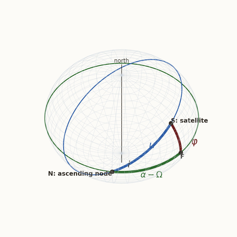
Reading Equation 17 gives the first properties of every circular ground track.
The largest latitude equals the inclination. \(\sin\varphi\le\sin i\), so \(|\varphi|_{\max}=i\) for \(i\le90^\circ\) and \(180^\circ-i\) for a retrograde orbit. The track lies between these parallels and touches them once per orbit (Figure 17, dashed lines). A polar orbit reaches the poles; an equatorial orbit never leaves the equator.
The track shifts west by \(\omega_\oplus T\) on every orbit. After one period \(u\) has increased by \(2\pi\) but \(\theta\) by \(\omega_\oplus T\), so the next equator crossing is displaced by \(-\omega_\oplus T\) in longitude: \[ \Delta\lambda_{\rm orbit}=-\omega_\oplus T=-360^\circ\frac{T}{T_{\rm sid}}\ \ (\text{with }J_2:\ -(\omega_\oplus-\dot\Omega)\,T_\Omega). \tag{18}\] For \(T=92.97\) min (the ISS) this is \(23.3^\circ\), i.e. \(2594\) km at the equator; for a \(650\) km orbit \(24.5^\circ\) (\(2727\) km). The number of orbits per day is \(86\,400/T\): \(15.49\) for the ISS.
The heading at the equator is not the inclination. At the ascending node \(u=0\), \(\dot\varphi=n\sin i\) and \(\dot\lambda=n\cos i-\omega_\oplus\), so the track crosses the equator at an angle \(\beta\) (measured from east) with \[ \tan\beta=\frac{n\sin i}{n\cos i-\omega_\oplus}. \tag{19}\] For the ISS (\(\omega_\oplus/n=0.0647\), \(i=51.64^\circ\)) this gives \(\beta=54.7^\circ\), steeper than the inertial \(51.64^\circ\): the surface is moving eastward under the satellite. For a retrograde orbit the Earth’s rotation adds to the westward motion, and for a geostationary orbit (\(n=\omega_\oplus\), \(i=0\)) the numerator and the denominator both vanish and the track collapses to a point.
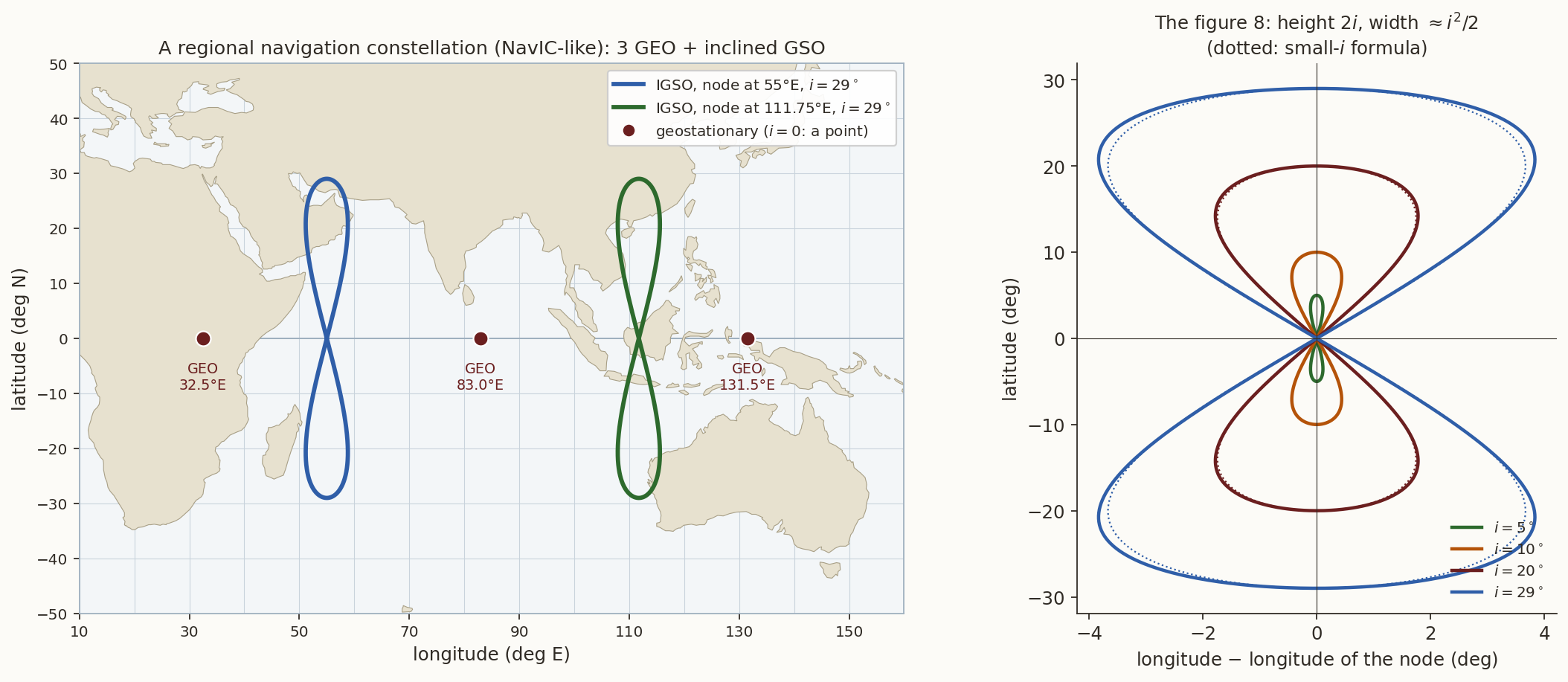
Small inclination at the geosynchronous radius gives a figure 8. If \(n=\omega_\oplus\) (the orbit is geosynchronous) then \(\lambda=\Omega+\bigl[\operatorname{atan2}(\cos i\sin u,\cos u)-u\bigr]\) and, for small \(i\), \(\operatorname{atan2}(\cos i\sin u,\cos u)-u\approx-\tfrac{i^2}{4}\sin2u\). The track is \[ \varphi=i\sin u,\qquad \lambda-\Omega\approx-\frac{i^{2}}{4}\sin2u, \tag{20}\] a figure 8 of height \(2i\) and width \(i^2/2\), traversed once per sidereal day (Figure 20, right, dotted: Equation 20). For \(i=29^\circ\) the exact longitude excursion is \(\pm3.84^\circ\) and Equation 20 gives \(\pm3.67^\circ\); for \(i=10^\circ\), \(\pm0.439^\circ\) against \(\pm0.436^\circ\).
2.2.2 The effect of \(J_2\), and mean against osculating elements
Over many orbits the equatorial bulge (see Beyond the Point Mass) turns the orbit plane and rotates the perigee, and changes the mean motion. The secular rates, with \(p=a(1-e^2)\), are \[ \dot\Omega=-\tfrac32 nJ_2\Bigl(\frac{R_\oplus}{p}\Bigr)^{2}\cos i,\quad \dot\omega=\tfrac34 nJ_2\Bigl(\frac{R_\oplus}{p}\Bigr)^{2}(5\cos^2 i-1),\quad \dot M=n\Bigl[1+\tfrac34J_2\Bigl(\frac{R_\oplus}{p}\Bigr)^{2}\sqrt{1-e^2}\,(3\cos^2i-1)\Bigr]. \tag{21}\] To include \(J_2\) in the ground track, replace \(M\), \(\Omega\), \(\omega\) in steps 2 to 4 by \(M_0+\dot Mt\), \(\Omega_0+\dot\Omega t\), \(\omega_0+\dot\omega t\). The node drift changes Equation 18 as shown, and it is what makes sun-synchronous orbits possible (Section 2.3.3).
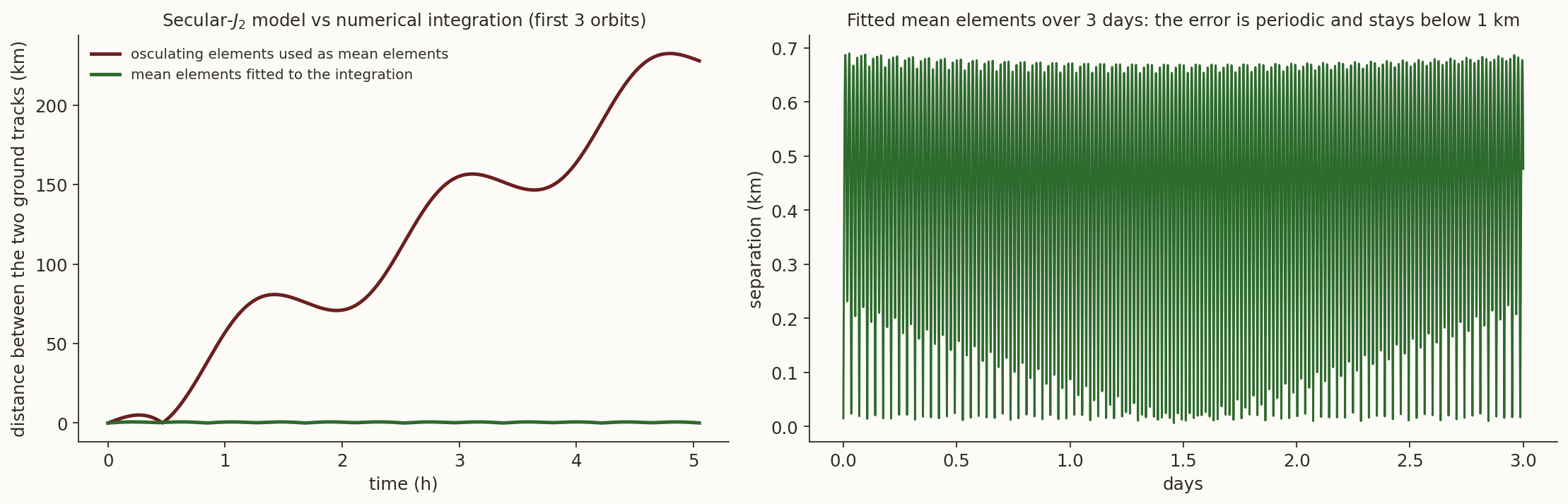
There is one trap. The rates of Equation 21 hold for mean elements: the elements averaged over an orbit. The osculating elements computed from an instantaneous position and velocity oscillate around them with amplitude \(\sim J_2R_\oplus^2/a\), which is about \(9\) km in \(a\) for a low orbit. Figure 16 makes the point. We integrated the equations of motion with the \(J_2\) acceleration for three days (DOP853, relative tolerance \(10^{-11}\)) for an \(800\) km orbit at \(i=98.6^\circ\), and compared with the analytic ground track. If the osculating elements at \(t=0\) are used as mean elements, the two tracks are \(76\) km apart after one orbit, \(1057\) km after a day and \(3256\) km after three days: the wrong semi-major axis (osculating \(7178.1\) km, mean \(7187.2\) km) makes the satellite run early. If the mean elements are fitted to the integration, the analytic track follows the integrated one to \(0.48\) km rms and \(0.69\) km at most over three days. The lesson is the standard one of mission analysis: use mean elements to describe orbits over long periods, and never mix them with osculating ones.
2.3 The standard ground tracks
2.3.1 Low Earth orbit
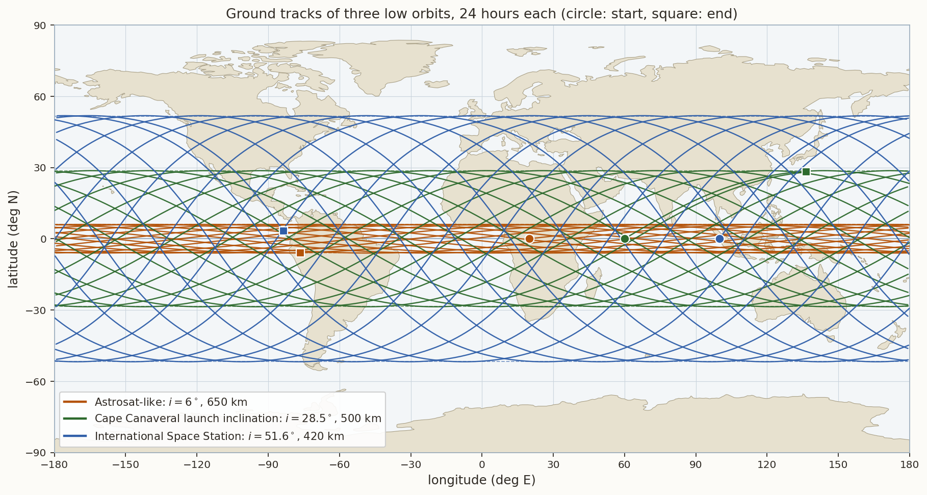
Figure 17 shows one day of three low orbits: a near-equatorial one (like India’s Astrosat, \(i=6^\circ\), \(650\) km), one at \(28.5^\circ\) (the latitude of Cape Canaveral, the lowest inclination reachable from there without a plane change), and the International Space Station (\(51.6^\circ\), \(420\) km). All three follow Equation 17: a sinusoid-like curve confined to the band \(|\varphi|\le i\), shifted west by \(23\) to \(25^\circ\) on every orbit. In a day the ISS completes \(15.5\) orbits and passes over every point between \(51.6^\circ\)N and \(51.6^\circ\)S; it never sees the poles.
2.3.2 Polar orbit
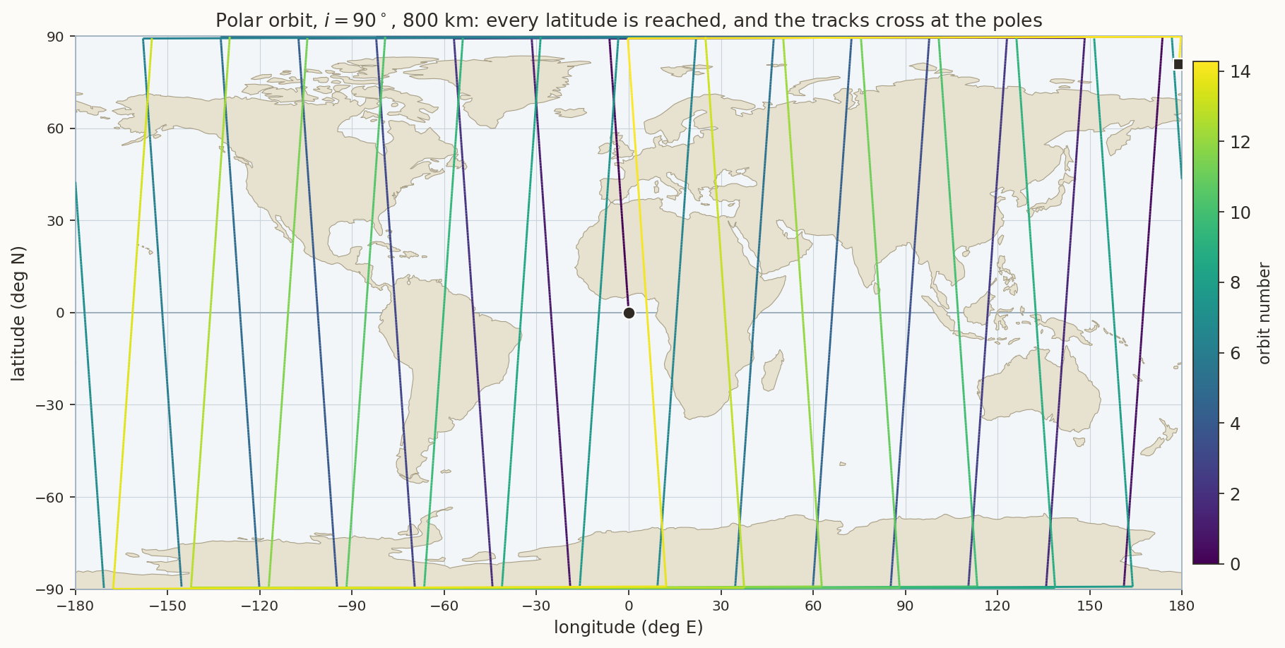
A polar orbit (\(i=90^\circ\)) passes over both poles on every revolution and, as the Earth turns underneath, eventually over every point on the globe (Figure 18). At \(800\) km the period is \(100.9\) min, there are \(14.3\) orbits per day, and successive tracks are \(25.3^\circ\) (\(2800\) km) apart at the equator. All tracks cross at the poles, so coverage is dense at high latitudes and sparsest at the equator. With \(J_2\) a polar orbit has \(\dot\Omega=0\): its plane stays fixed in inertial space, so relative to the Sun it turns once a year.
2.3.3 Sun-synchronous orbit
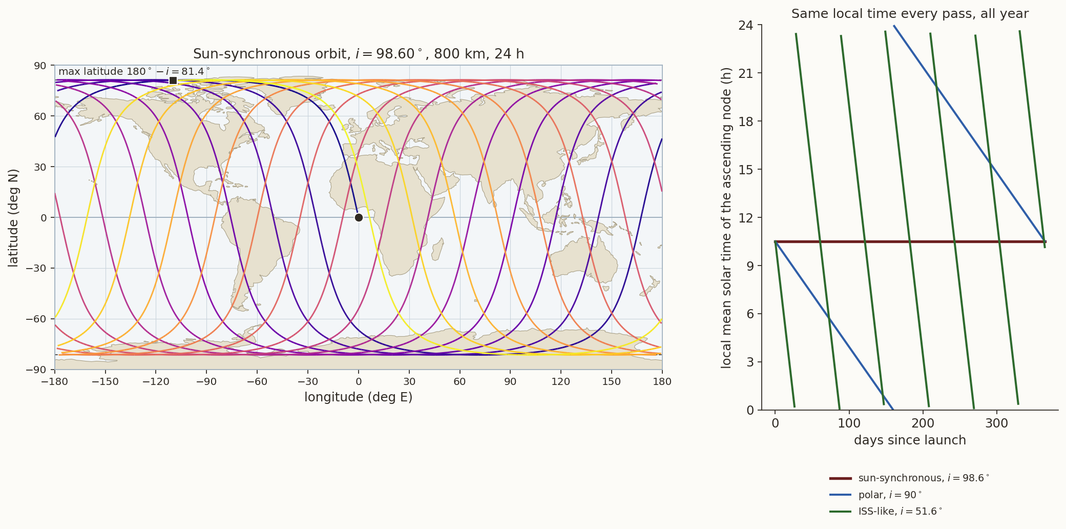
A sun-synchronous orbit (SSO) is not an orbit that follows the Sun. It is an orbit whose plane turns at exactly the rate at which the Sun’s right ascension increases, \[ \dot\Omega=\frac{2\pi}{365.2422\ \text{d}}=+0.98565^\circ/\text{day}, \tag{22}\] so that the angle between the orbit plane and the Earth–Sun line never changes. The satellite then crosses the equator at the same local mean solar time on every pass for the whole mission, which means the same sun elevation, the same shadow lengths and an unchanging power and thermal environment.
Equation 21 gives \(\dot\Omega\propto-\cos i\), and Equation 22 needs \(\dot\Omega>0\), so every sun-synchronous orbit is retrograde. Solving \(\dot\Omega=0.98565^\circ\)/day for the inclination gives, for circular orbits, \(i=98.60^\circ\) at \(800\) km and \(i=98.19^\circ\) at \(700\) km. The highest latitude is then \(180^\circ-i=81.4^\circ\), so an SSO covers the whole globe except for small polar caps. The right panel of Figure 19 shows the payoff: the local time of the ascending node stays constant for a year, whereas a polar orbit (fixed plane) drifts through \(24\) h in a year (\(-1.97\) h per \(30\) days) and the ISS orbit through \(24\) h in about \(2.5\) months (\(-11.9\) h per \(30\) days).
History. The first Earth-observation satellite in a sun-synchronous orbit of the kind we use today was Landsat 1 (launched in 1972, then called ERTS-1; \(917\) km, \(99.1^\circ\)). Since then it has been the standard orbit for imaging, because the same local time gives comparable lighting from one pass to the next; a mid-morning descending node (about \(10{:}30\)) balances haze and shadows for optical imaging, a dawn-dusk orbit keeps the arrays in nearly continuous sunlight.
2.3.4 Geostationary and geosynchronous orbits
At \(a=42\,164\) km (\(T=\) one sidereal day) and \(i=0\) the sub-satellite point is fixed: the geostationary orbit is the only orbit whose ground track is a point. Its ground track is a single dot, and a single dot is exactly what a communications or weather satellite wants: a ground antenna does not have to move. At this altitude a satellite sees \(42\%\) of the surface (Section 2.5), so three satellites cover the equatorial and mid-latitude world.
If the same orbit is inclined (\(i>0\)) it is geosynchronous but no longer stationary: the sub-satellite point traces the figure 8 of Equation 20, once a day (Figure 20). India’s regional navigation system NavIC uses exactly this combination: three geostationary satellites (at \(32.5^\circ\)E, \(83^\circ\)E and \(131.5^\circ\)E) and four inclined geosynchronous ones (\(i=29^\circ\)) whose figures of eight are centred at \(55^\circ\)E and \(111.75^\circ\)E, so that at any moment several satellites are high in the sky over India. Historically, Syncom 2 (1963), the first geosynchronous satellite, had an inclination of \(33^\circ\) and drew a figure 8 before Syncom 3 (1964) became the first geostationary one.
2.3.5 Highly elliptical orbits: Molniya and Tundra
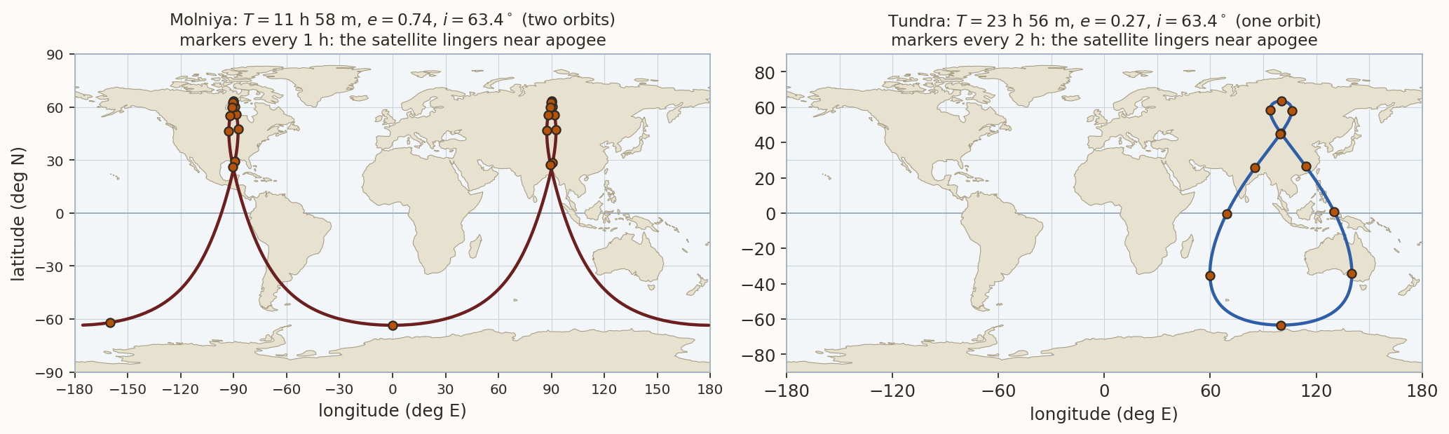
For \(e>0\) the satellite is not uniformly fast: by Kepler’s second law it lingers near apogee. The Molniya orbit (\(T=\) half a sidereal day, \(e=0.74\), \(a=26\,562\) km, perigee altitude \(528\) km, apogee altitude \(39\,840\) km) exploits this. Its inclination is \(i=63.4^\circ\), the critical inclination \(\arccos(1/\sqrt5)\) at which \(\dot\omega=0\) in Equation 21, so the apogee stays over the northern hemisphere instead of rotating away. The satellite is above \(55^\circ\)N for \(6.2\) h of each \(12\) h orbit, and the speed at perigee is \(6.7\) times that at apogee (Figure 21, dots are one hour apart). Two such orbits per day put apogee alternately over Russia (\(90^\circ\)E in the figure) and over North America. Geostationary satellites at high latitude are near the horizon; a Molniya satellite is almost overhead. The Tundra orbit (\(T\) = one sidereal day, \(e\approx0.27\), same inclination) gives a figure 8 with a small northern loop that dwells over one region for many hours.
History. The first Molniya satellite was launched in April 1965. The reasoning was geometric: geostationary satellites are near the horizon at the high latitudes of the Soviet Union, and the highly elliptical orbit at the critical inclination is the cheapest way to stay high in the sky for most of the day.
2.3.6 Repeat ground tracks
A ground track repeats if, after \(k\) revolutions, the Earth has turned through a whole number \(D\) of complete turns relative to the orbit plane. Between two successive ascending nodes, the Earth turns relative to the plane through \((\omega_\oplus-\dot\Omega)\,T_\Omega\), where \(T_\Omega=2\pi/\dot u\) is the nodal period (\(\dot u=\dot M+\dot\omega\) is the rate of the argument of latitude). Repeat after \(k\) orbits and \(D\) turns means \[ k\,(\omega_\oplus-\dot\Omega)\,T_\Omega=2\pi D \quad\Longleftrightarrow\quad \boxed{\ \frac{\dot M+\dot\omega}{\omega_\oplus-\dot\Omega}=\frac kD\ } \tag{23}\] with \(k\), \(D\) integers without common factor. With \(J_2\) neglected this reads \(n\,T_{\rm sid}=2\pi k/D\), i.e. \(T=(D/k)\,T_{\rm sid}\). The left-hand side of Equation 23 depends on \(a\) (and weakly on \(e\) and \(i\)), so for given \(k\), \(D\), \(i\), \(e\) it is solved for \(a\) by bisection. The ground track repeats after \(D\) nodal days, \(2\pi/(\omega_\oplus-\dot\Omega)\) each. For a sun-synchronous orbit \(\omega_\oplus-\dot\Omega\) is exactly \(2\pi\) per mean solar day, so the nodal day is the solar day (Section 1.2.2) and the cycle is \(D\) solar days; for a geosynchronous or GPS orbit \(\dot\Omega\) is tiny and the nodal day is very nearly the sidereal day.
After the cycle the \(k\) ascending nodes are equally spaced around the equator, \(360^\circ/k\) apart: the tracks fill in a grid with spacing \(2\pi R_\oplus/k\) at the equator. This is the design equation of an Earth-observation mission: choose \(k\) so that the spacing is a little less than the swath of the instrument.
We tested the solver against orbits whose parameters are published (Table 7): the agreement is a check on the whole chain of Equation 21 and Equation 23.
| Mission | \(k/D\) | Computed \(a-R_\oplus\) | Published |
|---|---|---|---|
| Sentinel-1 (SSO) | \(175/12\) | \(692.8\) km | \(693\) km |
| Sentinel-2 (SSO) | \(143/10\) | \(786.1\) km | \(786\) km |
| Resourcesat / IRS-1C (SSO) | \(341/24\) | \(817.0\) km | \(817\) km |
| Landsat 8, 9 (SSO) | \(233/16\) | \(699.6\) km | \(705\) km (osculating, at the equator) |
| Jason-3 (\(66.04^\circ\)) | \(127/10\) nodal days | \(1336.3\) km, cycle \(9.9156\) solar d | \(1336\) km, \(9.9156\) d |
| GPS (\(55^\circ\)) | \(2/1\) | \(20\,182.3\) km, \(a=26\,560.4\) km | \(a=26\,560\) km |
| Galileo (\(56^\circ\)) | \(17/10\) | \(a=29\,600.3\) km | \(a=29\,600\) km |
| GLONASS (\(64.8^\circ\)) | \(17/8\) | \(a=25\,507.6\) km | \(a=25\,508\) km |
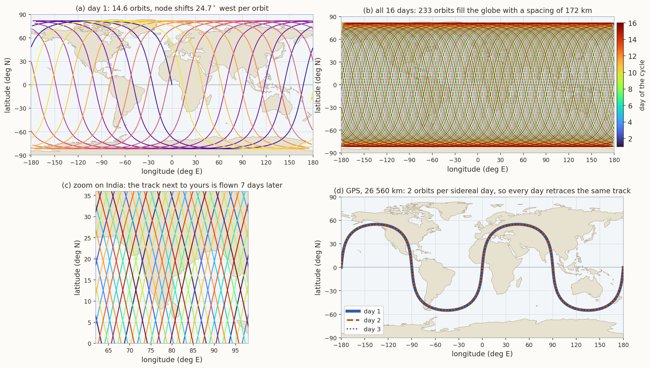
The left panels of Figure 22 show the Landsat-like orbit. It flies \(14.56\) orbits per day, the ascending nodes advance \(24.72^\circ\) westward per orbit, and after \(16\) days the \(233\) tracks are spaced \(1.545^\circ=172.0\) km apart at the equator. The instrument swath of \(185\) km then gives a sidelap of \((185-172)/185=7\%\) at the equator, which grows toward the poles. Neighbouring tracks are flown seven days apart (modulo the \(16\)-day cycle), which is why a place is not re-imaged for a week after its neighbour. Panel (d) shows the case of GPS: two orbits per sidereal day, so that each day retraces the same path over the ground.
History. The altimetry satellite TOPEX/Poseidon (1992) was given a \(9.9156\)-day repeat cycle (\(127\) orbits) so that the tidal constituents, which are aliased by the sampling, appear at distinct periods (the lunar \(M_2\) tide is aliased to about \(62\) days) and can be separated from the slow sea-level changes that the mission was after. Jason-1, -2 and -3 fly the same ground track.
2.4 An interactive ground-track simulator
The figure below implements the six steps of Section 2.2 in JavaScript, in the browser. Pick a preset, or change the elements with the sliders (or type exact values into the boxes), and the ground track is redrawn. Press play to fly the satellite along its track with its footprint. Tick ground station to see the passes. The panel of read-outs gives the derived quantities of this note: period, nodal drift, shift per orbit, and, if the orbit repeats, the ratio of Equation 23.
Things to try (each takes a minute and each answers a question of this note).
- ISS. Play the preset for a day. How many orbits does it make? How far west does the track move on each orbit (read-out)? Compare with Equation 18.
- Geostationary, then increase \(i\) from \(0\) to \(29^\circ\) in small steps. Watch the point become a figure 8. Reproduce Equation 20.
- A 24-hour orbit. Set the preset “A 24-hour orbit”. The track is a straight line along the equator, running west at \(0.9856^\circ\)/day (Figure 4). Change \(a\) to \(42\,164.17\) km to stop it.
- Sun-synchronous. Take the SSO preset, untick \(J_2\): the node no longer moves and the local time of the pass is not constant. Tick it again and change \(i\) by \(0.5^\circ\): the read-out shows the drift \(\dot\Omega\) leaving \(0.9856^\circ\)/day.
- Repeat orbit. Press solve for a with \(k=233\), \(D=16\) (sun-synchronous ticked). Play the \(16\)-day cycle. Then type \(k=15\), \(D=1\) with the box unticked: an orbit with \(15\) revolutions per (nodal) day.
- Molniya. Set \(\omega=270^\circ\), then \(\omega=200^\circ\) and compare. Untick \(J_2\) and see that the apogee stays where it is only at the critical inclination \(i=63.4^\circ\).
- A station. Tick ground station at \((13.0^\circ\mathrm N,\,77.6^\circ\mathrm E)\) and read the passes of the SSO preset. Then move the station to Svalbard (\(78.2^\circ\)N, \(15.4^\circ\)E): how many passes per day now?
2.5 What ground tracks are used for
| Application | Orbit | Ground-track property used | Example |
|---|---|---|---|
| Optical / radar Earth observation | sun-synchronous, repeat orbit | same local time every pass; global coverage; track spacing \(<\) swath | Landsat, Sentinel, Resourcesat |
| Altimetry | non-sun-synchronous, exact repeat | repeat cycle with aliasing of tides | TOPEX/Poseidon, Jason |
| Continuous regional service | geostationary | fixed sub-satellite point | INSAT, GOES, Meteosat |
| Regional navigation | GEO + inclined geosynchronous | figure 8 over the region | NavIC, QZSS, BeiDou |
| High-latitude communication | Molniya, Tundra | slow near apogee over the north | Molniya, Sirius XM |
| Global navigation | MEO, repeat every few days | track repeats every sidereal day (GPS), every 8–10 days (GLONASS, Galileo) | GPS, Galileo |
| Weather, global | polar / SSO | all latitudes, twice a day | Metop, NOAA |
| Crew and cargo | ISS, \(51.6^\circ\) | visible from most populated latitudes; launch from mid-latitude sites | ISS |
2.5.1 Coverage: footprints and swaths
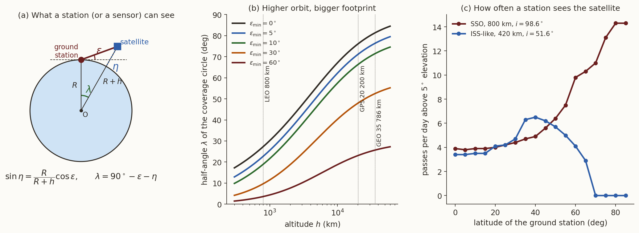
A satellite at altitude \(h\) sees, above a minimum elevation angle \(\varepsilon\), a circle on the ground of angular radius \(\lambda\) (the Earth central angle) around the sub-satellite point (Figure 24, left). From the triangle Earth centre–station–satellite, \[ \sin\eta=\frac{R_\oplus}{R_\oplus+h}\cos\varepsilon,\qquad \lambda=90^\circ-\varepsilon-\eta , \tag{24}\] where \(\eta\) is the nadir angle at which the station is seen from the satellite. At \(800\) km with \(\varepsilon=10^\circ\) the coverage radius is \(\lambda=18.95^\circ\) (\(2109\) km); at \(\varepsilon=0\) it is \(27.3^\circ\). For a geostationary satellite \(\lambda=81.3^\circ\) at \(\varepsilon=0\): it sees \(\tfrac12(1-\cos81.3^\circ)=42.4\%\) of the whole surface. Three of them, \(120^\circ\) apart, cover all longitudes up to a latitude of about \(\pm72^\circ\) at \(\varepsilon=0\), and about \(\pm62^\circ\) if \(5^\circ\) of elevation is required. For an imaging satellite the footprint is the instrument swath, about \(100\) to \(200\) km, and the ground track is its centre line: the design condition is the spacing of the repeat grid (Equation 23) against the swath.
2.5.2 Ground stations: how often, and for how long
The same equation gives the contact with a ground station: the satellite is visible when its sub-satellite point is within \(\lambda\) of the station (Figure 24, right; the dashed circle in the simulator). We counted passes above \(5^\circ\) elevation over ten days by direct computation (Table 9).
| Station | SSO \(800\) km: passes/day | contact min/day | min per pass | ISS: passes/day | contact min/day |
|---|---|---|---|---|---|
| Equator | \(3.9\) | \(37\) | \(9.5\) | \(3.4\) | \(23\) |
| Thiruvananthapuram (\(8.5^\circ\)N) | \(3.7\) | \(37\) | \(10.0\) | \(3.6\) | \(23\) |
| Bengaluru (\(13.0^\circ\)N) | \(3.8\) | \(37\) | \(9.8\) | \(3.6\) | \(24\) |
| Delhi (\(28.6^\circ\)N) | \(4.3\) | \(42\) | \(9.8\) | \(4.6\) | \(30\) |
| Svalbard (\(78.2^\circ\)N) | \(14.3\) | \(156\) | \(10.9\) | \(0\) | \(0\) |
A polar-type orbit passes near the poles on every one of its \(14.3\) orbits per day, so a station at \(78^\circ\)N is in contact on every orbit: this is why polar-orbit missions use high-latitude stations for data download. A station at low latitude sees such a satellite only three to four times a day, each pass lasting about ten minutes. The ISS never rises above \(5^\circ\) from Svalbard. Two practical numbers follow: a low-latitude station can download a few tens of minutes of data per day from a polar LEO satellite (which is why on-board storage and a high-latitude station matter), and a low-inclination LEO satellite is best served by stations near its maximum latitude.
2.5.3 The launch site sets the lowest inclination
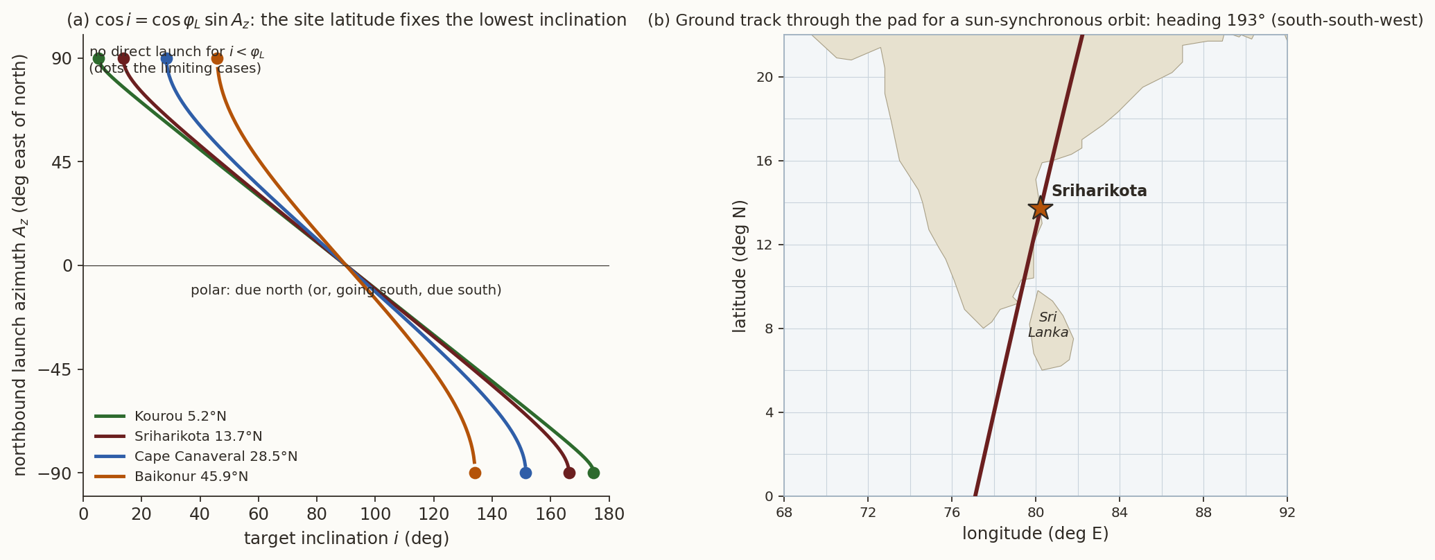
A launch vehicle can put a satellite directly into an orbit of inclination \(i\) only if \(i\ge\varphi_L\), the latitude of the launch site, because the orbit plane contains the Earth’s centre and the launch point, so it reaches at least latitude \(\varphi_L\). The launch azimuth \(A_z\) (from north, inertial) follows from the spherical triangle of Figure 15 applied to the launch point: \[ \cos i=\cos\varphi_L\,\sin A_z . \tag{25}\] A due-east launch (\(A_z=90^\circ\)) gives \(i=\varphi_L\) and also takes full advantage of the Earth’s rotation, which contributes \(\omega_\oplus R_\oplus\cos\varphi_L\) to the speed: \(463\) m/s at Kourou (\(5.2^\circ\)N), \(452\) m/s at Sriharikota (\(13.7^\circ\)N), \(409\) m/s at Cape Canaveral (\(28.5^\circ\)N), \(324\) m/s at Baikonur (\(45.9^\circ\)N). For a sun-synchronous orbit with \(i=98.7^\circ\) from Sriharikota, Equation 25 gives \(A_z\approx-9^\circ\) or \(189^\circ\): the vehicle flies almost due south, against the rotation of the Earth, and the ground track through the launch site heads \(193^\circ\), south-south-west, after the rotation of the Earth is taken out (Figure 25, right). This track passes close to the west coast of Sri Lanka, and avoiding an overflight of Sri Lanka is the reason usually given for the dog-leg manoeuvre that India’s PSLV flies on its sun-synchronous launches (the ascent path, unlike the final orbit’s track, is bent around the island; our figure shows only the orbit’s ground track through the pad).
Part 2 in one paragraph. The ground track is the inertial orbit seen from the rotating Earth: elements \(\to\) Kepler \(\to\) perifocal \(\to\) inertial \(\to\) rotate by \(\theta=\theta_0+\omega_\oplus t\) \(\to\) \((\varphi,\lambda)\). For circular orbits \(\sin\varphi=\sin i\sin u\) and \(\tan(\alpha-\Omega)=\cos i\tan u\): the highest latitude is \(i\), the track moves \(360^\circ\,T/T_{\rm sid}\) west per orbit, and near the geosynchronous radius a small inclination gives a figure 8 of width \(i^2/2\). \(J_2\) adds \(\dot\Omega\), \(\dot\omega\), \(\dot M\) (use mean elements!) and makes sun-synchronous orbits possible; the repeat condition is \((\dot M+\dot\omega)/(\omega_\oplus-\dot\Omega)=k/D\). Every application in Table 8 is a statement about one of these properties.
Summary and outlook
What we left out. (i) Precession, nutation and polar motion. The transformation from ECI to ECEF is here a single rotation. The full IAU 2006/2000A transformation adds precession, nutation and polar motion, which move points on the ground by up to a few hundred metres. (ii) Drag and other perturbations, which change \(a\) and hence the period and the repeat pattern: repeat-orbit missions carry propellant to hold the ground track within a tolerance band (typically \(\pm1\) km of the reference track for the Landsat series; check the mission documentation). (iii) The complete time scales, in particular the SPICE system used by space agencies, which handles the conversion between spacecraft clock, UTC, TDB and ephemeris time with kernels.
Further reading. H. D. Curtis, Orbital Mechanics for Engineering Students (Julian date, sidereal time, ground tracks); D. A. Vallado, Fundamentals of Astrodynamics and Applications (time scales, the IAU transformations, ground tracks and repeat orbits); the IERS Conventions (2010) and the Explanatory Supplement to the Astronomical Almanac for time scales and the equation of time; N. Ashby, Relativity in the Global Positioning System, Living Reviews in Relativity 6 (2003), for the GPS clock corrections; J. Taylor and colleagues at JPL on deep-space Doppler tracking and Allan deviation.
Exercises
Time
- Sidereal day. Use Equation 2 with the tropical year \(365.242189\) d to show that \(T_{\rm sid}=86\,164.0905\) s, and with the sidereal year \(365.256363\) d to obtain the stellar day to within about a millisecond. Why do the two answers differ by \(8.4\) ms?
- Revolutions per day. A satellite is in a circular orbit at \(400\) km altitude. How many revolutions does it make per solar day and per sidereal day? (Answers: \(T=5553.6\) s; \(15.56\) per solar day, \(15.52\) per sidereal day.)
- The 24-hour orbit. Derive the drift rate \(0.9856^\circ\)/day of a satellite in a circular equatorial orbit of period \(86\,400\) s from the ratio of the periods, and its semi-major axis.
- Launch window. The ISS has \(\dot\Omega=-4.95^\circ\)/day. By how many minutes does an instantaneous launch window move from one day to the next? (Answer: about \(24\) min earlier; the interval between windows is \(23.6\) h.)
- TDB. Verify the amplitude \(1.657\) ms of TDB \(-\) TT from Equation 6. What would the amplitude of the corresponding periodic term be for a clock on Mars (\(a=1.5237\) AU, \(e=0.0934\))? (Answer: about \(11\) ms, because the amplitude scales as \(\sqrt a\,e\).)
- Ranging. To what accuracy in ns must the round-trip time be measured for a \(1\) m range? Which clock class of Table 4 gives \(\delta\rho<1\) m at \(2.5\) AU? (Answer: \(6.7\) ns; rubidium is marginal at \(3.7\) m, caesium is sufficient.)
- Ledger. By how many kilometres is a \(500\) km satellite displaced along its orbit if GPS time is mistaken for UTC? (Answer: \(137\) km.)
Ground tracks
- Heading at the node. Evaluate Equation 19 for the ISS (\(T=92.97\) min, \(i=51.64^\circ\)). What is the heading for an SSO at \(800\) km? Why is it larger than \(90^\circ\)? (Answers: \(54.7^\circ\); \(102.5^\circ\), because the orbit is retrograde and the Earth’s rotation adds to the westward motion.)
- SSO design. Find the inclination of a circular sun-synchronous orbit at \(700\) km from \(\dot\Omega=0.9856^\circ\)/day. (Answer: \(98.19^\circ\).)
- Track spacing. For \(233\) orbits in \(16\) days, find the equatorial spacing of tracks in degrees and kilometres, and the sidelap of a \(185\) km swath. (Answers: \(1.545^\circ\), \(172\) km, \(7\%\).)
- Repeat orbit, no \(J_2\). Find the altitude of a circular orbit with \(15\) revolutions in one stellar day, neglecting \(J_2\). (Answer: about \(554\) km.)
- Figure 8. For a geosynchronous orbit with \(i=29^\circ\) find the width and height of the figure 8 from Equation 20, and compare with the exact value \(\pm3.84^\circ\) of the longitude excursion.
- Footprint. At what altitude does a satellite see an Earth central angle of \(\lambda=30^\circ\) at \(\varepsilon=10^\circ\)? Use Equation 24. (Answer: \(\eta=50^\circ\), \(R_\oplus+h=R_\oplus\cos10^\circ/\sin50^\circ\), \(h\approx1820\) km.)
- Launch. Which is the lowest inclination reachable directly from Kourou? From Baikonur? What is the northbound launch azimuth from Sriharikota into a \(98.6^\circ\) orbit? (Answers: \(5.2^\circ\); \(45.9^\circ\); \(-8.9^\circ\), i.e. \(351.1^\circ\).)
- Simulator. Using Section 2.4, find the altitude and inclination of a sun-synchronous orbit that repeats after \(D=16\) solar days with \(k=229\) orbits, and read off the spacing of the tracks (\(360^\circ/229=1.572^\circ\)). Why would \(k=232\), \(D=16\) not be a good choice? (Hint: \(\gcd(232,16)=8\).) (Answers: \(a=7160.1\) km, altitude \(781.9\) km, \(i=98.53^\circ\), spacing \(175\) km; \(232/16=29/2\) repeats after \(2\) days, not \(16\).)