The Impulsive Model
1 The impulsive model
The two-body note and the orbital-elements note taught us to describe an orbit and to follow a spacecraft along it. But a spacecraft is rarely content with the orbit it is given. A launcher may leave it in a low orbit when it has to reach geostationary height. It may arrive behind a space station and have to catch up. It may have to tilt its orbital plane, or leave the Earth altogether. All of these mean changing the orbit with a rocket engine.
So the question behind all the manoeuvre notes is the same. What is the smallest change of velocity that does the job, and where along the orbit should the engine fire? Before we can answer this for any particular manoeuvre, we need three things, and this note provides them. We need a simple model of a burn. We need to know how a change of velocity turns into propellant. And we need to know what one burn does to an orbit.
The course text treats the same material in chapter 6 (Curtis 2014). Symbols and constants shared by all the notes are on the notation page.
1.1 Burns as instantaneous impulses
A real engine burns for a finite time, and the spacecraft moves while it burns. This makes the motion hard to work out. To simplify it, we replace the burn by an instantaneous jump in velocity at a fixed point:
\[ \mathbf r^{+}=\mathbf r^{-},\qquad\mathbf v^{+}=\mathbf v^{-}+\Delta\mathbf v . \]
The superscripts \(-\) and \(+\) mean just before and just after the burn. We call this jump an impulse. With it, a manoeuvre becomes a set of ordinary two-body orbits joined at the burn points, and we already know how to work with those. The model is good when the burn lasts a small fraction of the orbital period \(T\), which means \(t_{\rm burn}/T\ll1\).
A chemical upper stage burns for a few minutes on an orbit whose period is hours. An ion engine produces about \(0.1\) N and must run for months to deliver the same \(\Delta v\). Is the impulsive model suitable for each?
Answer
For the chemical stage, \(t_{\rm burn}/T\) is a few percent, so the model is excellent. For the ion engine the burn spans hundreds of revolutions. There is no single point at which the impulse happens, and the path is a slow spiral. It has to be treated as a problem with continuous thrust.How good is the model in practice? The departure burn of ISRO’s Mangalyaan lasted \(1329\) s on an orbit with a period of about \(91\) h, so \(t_{\rm burn}/T\) was only \(0.4\%\). Even so, the flown burn was reported as \(648\) m/s, and the impulsive calculation in the escape note gives \(616\) m/s, which is about \(5\%\) less. The reason is that the burn was made at perigee, where the spacecraft was moving at about \(10.8\) km/s. It covered about \(14\,000\) km during the burn, so it did not stay at one point. So we should treat the impulsive cost as a lower estimate, and expect the real cost to be higher for a long burn close to the planet.
The cost of an impulse is the scalar \(\Delta v=|\Delta\mathbf v|\). The cost of a sequence of burns is the sum of the sizes, \(\sum_i|\Delta\mathbf v_i|\), and not the size of the vector sum. Two burns that cancel each other still cost twice, because each one consumes propellant.
1.2 From \(\Delta v\) to propellant: the rocket equation
Why do we measure cost in \(\Delta v\) and not in propellant mass? Because the two are tied together by a law that does not depend on the manoeuvre. We will now derive it.
Consider a rocket of mass \(m\) in free space, which expels propellant at a speed \(v_e\) relative to itself. We call \(v_e\) the exhaust speed. In a short time \(dt\) the rocket ejects a mass \(-dm>0\) backwards and gains a speed \(dv\). Momentum is conserved. Before this time the momentum is \(mv\). After it, the rocket of mass \(m+dm\) moves at \(v+dv\), and the ejected mass \(-dm\) moves at \(v-v_e\). So
\[ mv=(m+dm)(v+dv)+(-dm)(v-v_e) . \]
Expanding and cancelling \(mv\) gives
\[ 0=m\,dv+v_e\,dm+dm\,dv . \]
The last term is a product of two small quantities, so we drop it. This leaves \(m\,dv=-v_e\,dm\). We separate the variables and integrate, with \(m_0\) and \(m_f\) the masses before and after the burn:
\[ \int_0^{\Delta v}dv=-v_e\int_{m_0}^{m_f}\frac{dm}{m}. \]
The result is
\[ \boxed{\;\Delta v=v_e\ln\frac{m_0}{m_f}=I_{sp}g_0\ln\frac{m_0}{m_f}, \qquad \frac{m_{\rm prop}}{m_0}=1-e^{-\Delta v/v_e}.\;} \tag{1}\]
Here \(I_{sp}=v_e/g_0\) is the specific impulse in seconds, with \(g_0=9.80665\) m/s\(^2\).
History: the rocket equation. It is usually credited to Konstantin Tsiolkovsky, who published it in 1903, although the same relation had been derived earlier in Britain (William Moore, 1813) for military rockets.
The fraction of the mass left after the burn is \(e^{-\Delta v/v_e}\), which falls exponentially with \(\Delta v\). So each extra km/s removes the same fraction of whatever is left. Table 1 shows this for \(I_{sp}=315\) s, for which \(v_e=3.089\) km/s.
| \(\Delta v\) (km/s) | \(1\) | \(2\) | \(4\) | \(8\) |
|---|---|---|---|---|
| Mass left | \(72.3\%\) | \(52.3\%\) | \(27.4\%\) | \(7.5\%\) |
Doubling \(\Delta v\) squares the fraction left. This is why a mission designer works hard to save even tens of metres per second, as the next example shows.
Example. A spacecraft must make a total \(\Delta v\) of \(3.8926\) km/s, which the Hohmann note shows is the cost of going from a \(300\) km circular orbit to the geostationary orbit. It uses ISRO’s \(440\) N liquid apogee motor, the main engine of Mangalyaan, with \(I_{sp}=315\) s. This is typical of storable-propellant engines worldwide. What fraction of the spacecraft’s mass at departure is propellant? If the spacecraft has a mass of \(3000\) kg at departure, how much more mass reaches the final orbit if we save \(50\) m/s?
Solution. The exhaust speed is \(v_e=315\times9.80665\times10^{-3}=3.0891\) km/s. So the fraction of propellant is
\[ \frac{m_{\rm prop}}{m_0}=1-e^{-3.8926/3.0891}=1-e^{-1.2601}=0.716 . \]
About \(72\%\) of the departure mass is propellant, and \(28.36\%\) reaches the final orbit. Saving \(50\) m/s raises this to \(e^{-3.8426/3.0891}=28.83\%\). On \(3000\) kg that is about \(14\) kg more mass delivered, a gain of \(1.6\%\). So a saving of just over \(1\%\) in \(\Delta v\) gives more than \(1\%\) in delivered mass, and all of this gain can go to the part of the spacecraft that does useful work.
1.3 What a single impulse does
Now we ask how an impulse changes an orbit. The energy \(\varepsilon=v^2/2-\mu/r\) and the angular momentum \(\mathbf h=\mathbf r\times\mathbf v\) fix the size and the shape of the orbit, so we look at how an impulse changes these two. An impulse \(\Delta\mathbf v\) does not change \(\mathbf r\). So the term \(\mu/r\) stays the same, and
\[ \varepsilon^{+}-\varepsilon^{-}=\frac{|\mathbf v+\Delta\mathbf v|^2}{2}-\frac{v^2}{2} =\mathbf v\cdot\Delta\mathbf v+\frac12|\Delta\mathbf v|^2 . \]
Also \(\mathbf h^{+}-\mathbf h^{-}=\mathbf r\times\Delta\mathbf v\). Writing \(\beta\) for the angle between \(\Delta\mathbf v\) and \(\mathbf v\),
\[ \boxed{\;\Delta\varepsilon=v\,\Delta v\cos\beta+\tfrac12\Delta v^2,\qquad\Delta\mathbf h=\mathbf r\times\Delta\mathbf v .\;} \tag{2}\]
Most of what we need in the later notes comes from reading these two formulas slowly.
The direction of the burn. For a fixed \(\Delta v\), the energy gain is largest when \(\beta=0\). So to change the energy, we burn along the velocity. We call this a tangential burn.
The place of the burn. The first term of \(\Delta\varepsilon\) has the factor \(v\). So the same \(\Delta v\) adds more energy where the spacecraft is already moving fast, and on an orbit that means at periapsis. This is called the Oberth effect. It follows that the \(\Delta v\) for a small energy change is approximately \(\Delta\varepsilon/v\).
A radial burn. If \(\Delta\mathbf v\) is along \(\mathbf r\), then \(\mathbf r\times\Delta\mathbf v=\mathbf 0\) and \(\mathbf h\) does not change. So \(p=h^2/\mu\) stays the same, and only \(e\) and the direction of the apse line can change. The apse-line note uses this. On a circle or at an apsis, a radial burn is also perpendicular to \(\mathbf v\), so \(\beta=90^\circ\) and it changes \(\varepsilon\) only through the small term \(\tfrac12\Delta v^2\). Elsewhere it changes \(\varepsilon\) at first order as well, by \(v_r\,\Delta v\), where \(v_r\) is the radial speed.
An out-of-plane burn. A burn with a component perpendicular to the orbital plane rotates \(\mathbf h\), which tilts the plane. Suppose that it only turns the velocity through an angle \(\theta\) and leaves the speed the same. The energy does not change at all. The velocities before and after, and the impulse between them, form an isosceles triangle with two equal sides of length \(v\) and the angle \(\theta\) between them. Its third side is the cost,
\[ \Delta v=2v\sin\frac\theta2 . \]
Example. An orbit has \(a=12\,000\) km and \(e=0.5\), with \(\mu=398\,600.4418\) km\(^3\)/s\(^2\). A tangential impulse of \(100\) m/s is applied. Find the energy it adds if it is applied at periapsis, and if it is applied at apoapsis.
Solution. Vis-viva gives the speeds at the two apsides:
\[ v_p=\sqrt{\frac{\mu}{a}\,\frac{1+e}{1-e}}=9.982\text{ km/s},\qquad v_a=\sqrt{\frac{\mu}{a}\,\frac{1-e}{1+e}}=3.327\text{ km/s}. \]
With \(\beta=0\) and \(\Delta v=0.1\) km/s, Equation 2 gives \(\Delta\varepsilon=v\,\Delta v+\tfrac12\Delta v^2\). The result is \(1.003\) km\(^2\)/s\(^2\) at periapsis and \(0.338\) km\(^2\)/s\(^2\) at apoapsis. So the burn at periapsis adds very nearly three times as much energy. The ratio of the speeds is \(v_p/v_a=(1+e)/(1-e)=3\), and the small term \(\tfrac12\Delta v^2\) is the same at both.
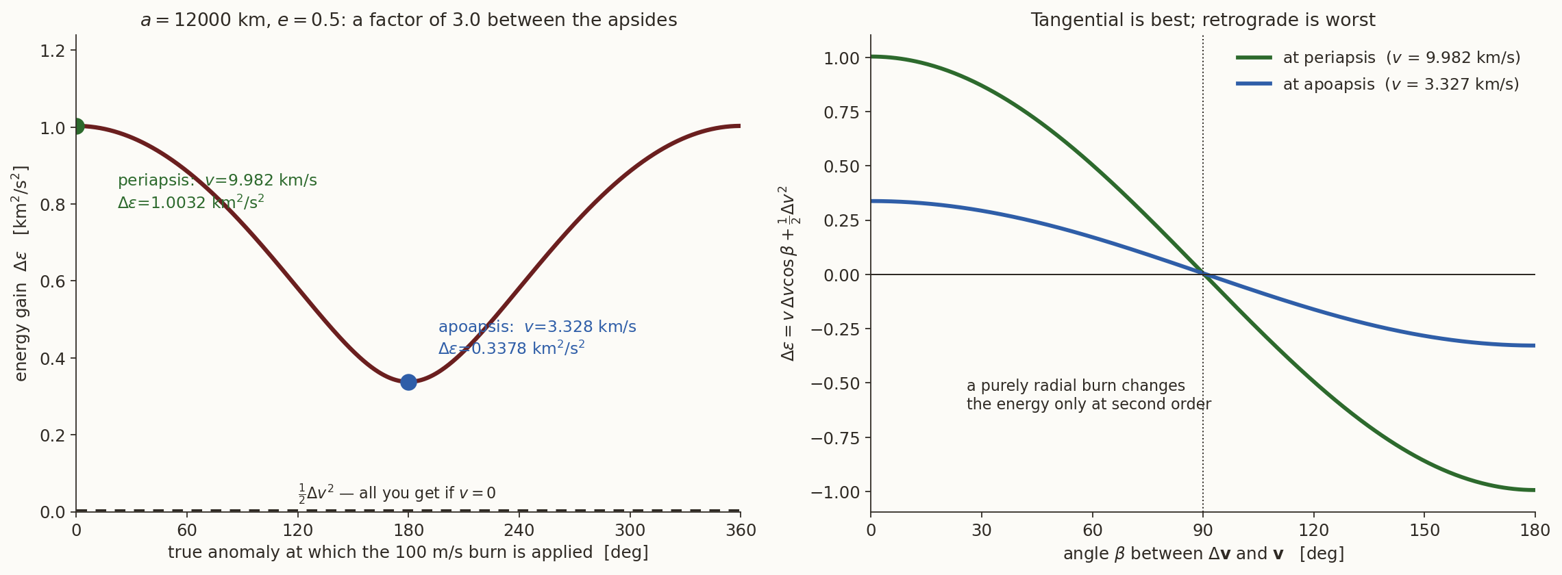
Figure 1 shows the whole picture. On the left is the energy added against the true anomaly of the burn, which varies smoothly between the values at the two apsides. On the right is the energy added against the direction of the burn. It varies as \(\cos\beta\), so a tangential burn adds the most, and a burn perpendicular to the velocity adds almost nothing.
We now have two results that pull in opposite directions. Energy is cheapest to change where \(v\) is large. The direction of the velocity is cheapest to change where \(v\) is small, since the cost is \(2v\sin(\theta/2)\). Most of the designs in the notes that follow are ways of dealing with this conflict. So transfers burn tangentially at periapsis where they can, and plane changes are made at apoapsis, where \(v\) is small.
There is a practical caution here too. A burn at periapsis has to wait for periapsis, which may be up to half a period away. So there is often a trade-off between propellant and time, and we will meet it in several of the notes that follow.
Each manoeuvre has its own note.
- The Hohmann transfer, including transfers between ellipses and why Hohmann is optimal
- The bi-elliptic transfer
- Phasing
- Rotating the apse line
- Plane changes
- Escape
2 Summary and exercise
We model a burn as an instantaneous change of velocity at a fixed point, and its cost is the size of that change. Propellant grows exponentially with the total \(\Delta v\) (Equation 1). A burn adds energy at a rate proportional to the speed \(v\) (Equation 2), so energy is cheapest to change at high speed. Turning the velocity costs \(2v\sin(\theta/2)\), so turning is cheapest at low speed.
- Rocket equation. A spacecraft with \(I_{sp}=320\) s must deliver \(5\) km/s of \(\Delta v\). What fraction of its initial mass is left at burnout? If its empty tanks are \(10\%\) of the initial mass, what fraction is payload? Now share the \(\Delta v\) equally between two stages of equal \(I_{sp}\), each with empty tanks equal to \(10\%\) of that stage’s initial mass (the stage and everything above it), the first being dropped before the second burns. What fraction is payload now? (Answers: \(20.3\%\), \(10.3\%\) and \(12.3\%\), so staging delivers \(19\%\) more payload.)
All the numbers in this note are checked by impulsive-model-verify.py.