Preliminary Orbit Determination
Where we are going
Every note so far began with the sentence “a satellite is at \(\mathbf r\) with velocity \(\mathbf v\)”. Nobody hands us that. What we have are measurements: a radar’s range and angles, a telescope’s right ascension and declination, a pair of GPS fixes. Orbit determination is the work of turning them into the six numbers that fix an orbit. It comes in two stages.
- Preliminary (or initial) orbit determination, the subject of most of this note, finds a state from the smallest set of observations that can determine it, with no first guess, using the two-body model and a few lines of algebra. The answer is rough, but it is all you have on the first pass over a new object.
- Refinement uses all the observations and a better dynamical model, and adjusts the state until the predicted observations match the measured ones as closely as possible, in the sense of least squares. It needs a first guess, and the preliminary answer is that guess. Section 9 gives the idea.
The preliminary methods are classified by what the observer measured:
| Data at each epoch | Method | Section |
|---|---|---|
| three positions at three times | Gibbs; Herrick–Gibbs when they are close | Section 2, Section 3 |
| two positions and the time between them | Lambert | Section 4 |
| three directions at three times (angles only) | Laplace; Gauss | Section 6, Section 7 |
| range, azimuth, elevation and their rates | direct conversion | topocentric note |
The background is the two-body problem, the orbital elements (the algorithm from a state to the elements is used at the end of every example), the Lagrange coefficients and Lambert solver of the universal-variables note, and, for the observations themselves, the topocentric note: the site vector, the right ascension and declination of a line of sight, and the warning that a topocentric direction is not a geocentric one. The note uses that note’s notation, and adds the symbols below. As elsewhere, a blue Try it box asks for a small calculation before you read on and a green Check yourself box asks a short question; each hides its answer.
| Symbol | Meaning |
|---|---|
| \(t_1,t_2,t_3\) | the three observation epochs; \(\tau_1=t_1-t_2<0\), \(\tau_3=t_3-t_2>0\), \(\tau=t_3-t_1\) |
| \(\mathbf r_i,\ \mathbf v_i\) | inertial position and velocity of the satellite at \(t_i\); \(r_i=\lVert\mathbf r_i\rVert\) |
| \(\mathbf R_i\) | inertial position of the station at \(t_i\): the site vector \(\mathbf r_{\rm site}\) of the topocentric note rotated through the Greenwich sidereal angle, \(\mathbf R_i=\mathbf R_3(\theta_G(t_i))\,\mathbf r_{\rm site}\) |
| \(\dot{\mathbf R},\ \ddot{\mathbf R}\) | velocity and acceleration of the station: \(\boldsymbol\omega_\oplus\times\mathbf R\) and \(\boldsymbol\omega_\oplus\times(\boldsymbol\omega_\oplus\times\mathbf R)\) (the site is fixed on the Earth, so only the rotation moves it) |
| \(\rho_i,\ \mathbf L_i\) | range from the station, and the unit line of sight in inertial components, \(\mathbf L_i\equiv\hat{\boldsymbol\rho}_i\) of the topocentric note; \(\mathbf r_i=\mathbf R_i+\rho_i\mathbf L_i\) |
| \(\alpha_i,\ \delta_i\) | topocentric right ascension and declination, \(\mathbf L_i=(\cos\delta_i\cos\alpha_i,\ \cos\delta_i\sin\alpha_i,\ \sin\delta_i)\) |
| \(F_i,\ G_i\) | Lagrange coefficients from \(t_2\) to \(t_i\): \(\mathbf r_i=F_i\mathbf r_2+G_i\mathbf v_2\) |
| \(p,\ \mathbf e,\ \mathbf h\) | semi-latus rectum, eccentricity vector (to periapsis), angular momentum |
1 What data do we need?
A two-body orbit is fixed by six numbers, so the observations must supply six independent numbers. The table of the introduction is just this count.
- A radar with Doppler gives \(\rho,A,\varepsilon\) and their rates, six numbers at one epoch. That is the state itself, and the topocentric note shows the conversion. Nothing more is needed.
- A position (three numbers) at one epoch is half a state; a second epoch of position gives six numbers, and the time between the two fixes closes the problem: that is Lambert’s. Three positions are nine numbers, more than needed, and Gibbs’s method uses them without the times.
- A direction (right ascension and declination) is two numbers; three epochs make six. At each epoch, one number is missing, the range \(\rho_i\). Three directions therefore determine the orbit only because the orbit is a Kepler orbit: the dynamics supply the three missing numbers. This is the hard case, and it is where most of the note goes.
1.1 The example used throughout
We know the truth in every example, so each method’s error can be reported (reality, of course, offers no such luxury). The station is Sriharikota, \(13.72^\circ\)N, \(80.23^\circ\)E, height \(10\) m. The epoch \(t=0\) is 14:00 UT on 14 October 2026, when the Greenwich sidereal angle is \(\theta_G=233.131^\circ\) (Curtis’s formula, as in the time note). The satellite moves on a two-body orbit with \[ \begin{aligned} a&=7800\ \text{km},\quad e=0.05826,\quad i=43.081^\circ,\\ \Omega&=290.224^\circ,\quad \omega=319.269^\circ,\quad f(0)=66.929^\circ, \end{aligned} \] so that the period is \(114.3\) min, the perigee radius is \(7345.5\) km and the apogee radius \(8254.5\) km. At \(t=0\), \[ \begin{aligned} \mathbf r(0)&=(4656.838,\ -5551.747,\ 2291.717)\ \text{km},\qquad r=7600\ \text{km},\\ \mathbf v(0)&=(3.621537,\ 4.413025,\ 4.604554)\ \text{km/s}. \end{aligned} \] The pass is shown in Figure 1. The satellite rises in the south-west, passes the station on its north-west side with a peak elevation of \(60.6^\circ\) (at \(t=-2\) s) and sets in the north-east: above \(10^\circ\) for \(927\) s, from \(t=-418\) s to \(t=+509\) s. At the five epochs we use, the station sees:
| \(t\) [s] | range [km] | azimuth | elevation | \(\alpha\) | \(\delta\) |
|---|---|---|---|---|---|
| \(-300\) | \(2269.593\) | \(245.333^\circ\) | \(20.887^\circ\) | \(249.4397^\circ\) | \(-17.1113^\circ\) |
| \(-60\) | \(1394.200\) | \(288.152^\circ\) | \(56.399^\circ\) | \(278.7186^\circ\) | \(21.4097^\circ\) |
| \(0\) | \(1370.344\) | \(320.697^\circ\) | \(60.603^\circ\) | \(291.0129^\circ\) | \(35.1436^\circ\) |
| \(+60\) | \(1449.817\) | \(351.649^\circ\) | \(56.185^\circ\) | \(306.7986^\circ\) | \(47.0505^\circ\) |
| \(+300\) | \(2410.785\) | \(30.931^\circ\) | \(25.355^\circ\) | \(18.0587^\circ\) | \(58.7162^\circ\) |
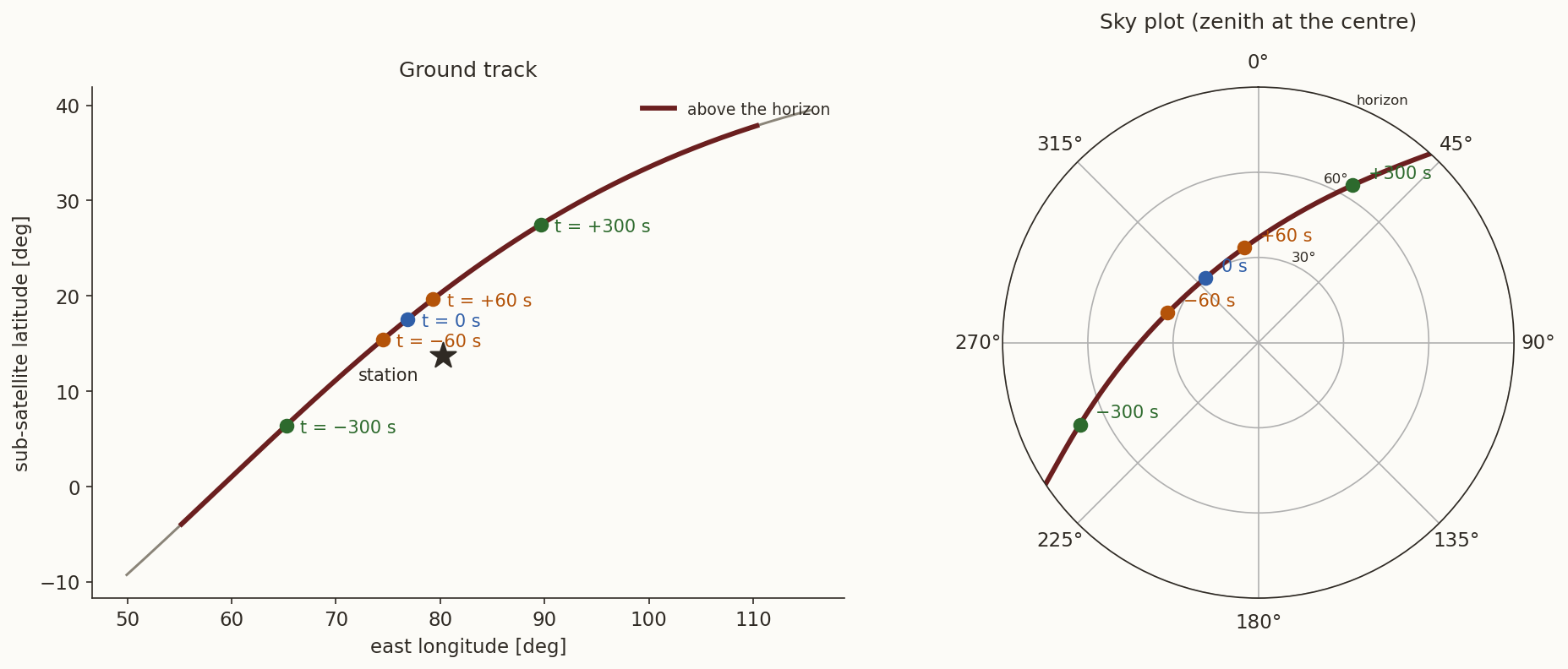
The azimuth, elevation and range of the table are computed with the helper module of the topocentric note (and checked against the line of sight built directly in inertial components by the verify script).
2 Three positions: the method of Gibbs
Suppose that a radar, or a pair of angle-and-range measurements converted with the topocentric note, has given the position of the satellite at three epochs, \(\mathbf r_1,\mathbf r_2,\mathbf r_3\), and that we want the velocity \(\mathbf v_2\) at the middle one. Gibbs’s method uses only geometry: three points on a conic with a focus at the origin fix the conic. The times do not enter at all.
History: Gibbs. J. Willard Gibbs (the physicist of thermodynamics and vector analysis) published a vector treatment of orbit determination in 1889 (Gibbs 1889). The step from three position vectors to the orbit, which is the method of this section, is the part of it that textbooks call Gibbs’s method. Writing everything with vectors, with no coordinates and no angles to unwind, is what makes it so short.
2.1 The conic as a linear equation
The orbit equation \(r=p/(1+e\cos f)\) is the same as \(r+e\,r\cos f=p\). Let \(\mathbf e\) be the eccentricity vector, of length \(e\), pointing from the focus to periapsis. Then \(e\,r\cos f=\mathbf e\cdot\mathbf r\), and
\[ r+\mathbf e\cdot\mathbf r=p . \tag{1}\]
This is a linear equation in the unknown vector \(\mathbf e\) and the unknown number \(p\), for every point of the orbit. At the three observed points,
\[ \mathbf e\cdot\mathbf r_i=p-r_i,\qquad i=1,2,3. \qquad\qquad (*) \]
The plan is to combine the three equations \((*)\) so as to eliminate \(\mathbf e\) and get \(p\), then to eliminate \(p\) and get \(\mathbf e\), and finally to get the velocity from \(p\) and \(\mathbf e\).
2.2 The three positions must be coplanar
All three points lie in the orbital plane, so each cross product \(\mathbf r_i\times\mathbf r_j\) is a multiple of the same unit vector \(\hat{\mathbf h}\): write \(\mathbf r_i\times\mathbf r_j=[ij]\,\hat{\mathbf h}\). Three vectors in a plane are linearly dependent, and the coefficients are exactly these brackets:
\[ [23]\,\mathbf r_1+[31]\,\mathbf r_2+[12]\,\mathbf r_3=\mathbf 0 . \tag{2}\]
To see it, call the left-hand side \(\mathbf V\) and cross it with \(\mathbf r_1\): since \(\mathbf r_2\times\mathbf r_1=-[12]\hat{\mathbf h}\) and \(\mathbf r_3\times\mathbf r_1=[31]\hat{\mathbf h}\), \(\mathbf V\times\mathbf r_1=-[31][12]\hat{\mathbf h}+[12][31]\hat{\mathbf h}=\mathbf 0\). In the same way \(\mathbf V\times\mathbf r_2=[23][12]\hat{\mathbf h}-[12][23]\hat{\mathbf h}=\mathbf 0\). A vector with zero cross product with two non-parallel vectors, \(\mathbf r_1\) and \(\mathbf r_2\), is zero, so \(\mathbf V=\mathbf 0\). (With noisy data the points are never exactly coplanar, and the size of \(\hat{\mathbf r}_1\cdot(\mathbf r_2\times\mathbf r_3)/\lVert\mathbf r_2\times\mathbf r_3\rVert\) is the natural test of the data: it is the sine of the angle by which \(\mathbf r_1\) leaves the plane of the other two.)
2.3 The semi-latus rectum
Dot Equation 2 with \(\mathbf e\) and use \((*)\):
\[ \begin{aligned} {}[23](p-r_1)+[31](p-r_2)+[12](p-r_3)&=0\\ \Longrightarrow\quad p\,\bigl([12]+[23]+[31]\bigr)&=r_1[23]+r_2[31]+r_3[12]. \end{aligned} \]
Multiplying by \(\hat{\mathbf h}\) turns the brackets back into vectors. Define
\[ \begin{aligned} \mathbf D&=\mathbf r_1\times\mathbf r_2+\mathbf r_2\times\mathbf r_3+\mathbf r_3\times\mathbf r_1,\\ \mathbf N&=r_1\,\mathbf r_2\times\mathbf r_3+r_2\,\mathbf r_3\times\mathbf r_1+r_3\,\mathbf r_1\times\mathbf r_2 , \end{aligned} \tag{3}\]
so that \(p\,\mathbf D=\mathbf N\). Both vectors point along \(\hat{\mathbf h}\), hence
\[ p=\frac{\lVert\mathbf N\rVert}{\lVert\mathbf D\rVert}. \tag{4}\]
2.4 The eccentricity vector
For the other combination we use the identity \((\mathbf a\times\mathbf b)\times\mathbf e=\mathbf b(\mathbf a\cdot\mathbf e)-\mathbf a(\mathbf b\cdot\mathbf e)\) and \((*)\):
\[ \begin{aligned} (\mathbf r_1\times\mathbf r_2)\times\mathbf e&=\mathbf r_2\,(\mathbf r_1\cdot\mathbf e)-\mathbf r_1\,(\mathbf r_2\cdot\mathbf e)\\ &=\mathbf r_2\,(p-r_1)-\mathbf r_1\,(p-r_2) =p\,(\mathbf r_2-\mathbf r_1)+r_2\,\mathbf r_1-r_1\,\mathbf r_2 . \end{aligned} \]
Add this to its two cyclic permutations. On the left, the three terms add to \(\mathbf D\times\mathbf e\). On the right, the terms in \(p\) cancel in the cyclic sum (\(\sum(\mathbf r_2-\mathbf r_1)=\mathbf 0\)), and what remains is
\[ \mathbf D\times\mathbf e=\mathbf S,\qquad \mathbf S=\mathbf r_1\,(r_2-r_3)+\mathbf r_2\,(r_3-r_1)+\mathbf r_3\,(r_1-r_2). \tag{5}\]
Since \(\mathbf e\) lies in the plane, it is perpendicular to \(\mathbf D\), and \(\mathbf D\times(\mathbf D\times\mathbf e)=-D^{2}\mathbf e\). So \(\mathbf D\times\mathbf S=-D^2\mathbf e\), that is
\[ \mathbf e=\frac{\mathbf S\times\mathbf D}{D^{2}} . \tag{6}\]
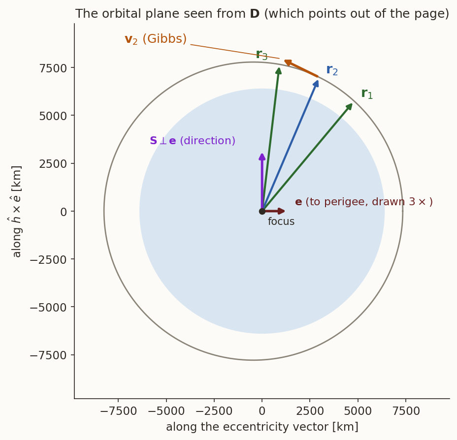
(For a circular orbit all \(r_i\) are equal, \(\mathbf S=\mathbf 0\) and \(\mathbf e=\mathbf 0\), as it should: Equation 5 contains the differences of the radii, which is what an eccentric orbit adds.) Figure 2 shows the vectors in the orbital plane: \(\mathbf S\) is perpendicular to \(\mathbf e\), because \(\mathbf D\times\mathbf e\) is.
2.5 The velocity
In the perifocal frame, with \(\hat{\mathbf P}\) along \(\mathbf e\) and \(\hat{\mathbf Q}=\hat{\mathbf h}\times\hat{\mathbf P}\), the velocity on a conic is \(\mathbf v=(\mu/h)\bigl[-\sin f\,\hat{\mathbf P}+(e+\cos f)\hat{\mathbf Q}\bigr]\) (the perifocal note derives it as the hodograph, a circle centred at \((0,e\mu/h)\)). Since \(\hat{\mathbf h}\times\hat{\mathbf P}=\hat{\mathbf Q}\), \(\hat{\mathbf h}\times\hat{\mathbf Q}=-\hat{\mathbf P}\), and \(\hat{\mathbf r}=\cos f\,\hat{\mathbf P}+\sin f\,\hat{\mathbf Q}\), the bracket is \(\hat{\mathbf h}\times(\mathbf e+\hat{\mathbf r})\):
\[ \mathbf v=\frac{\mu}{h}\ \hat{\mathbf h}\times(\mathbf e+\hat{\mathbf r}),\qquad h=\sqrt{\mu p}. \tag{7}\]
Now put in what we have. \(\hat{\mathbf h}=\mathbf D/D\), and by Equation 5, \(\hat{\mathbf h}\times\mathbf e=\mathbf S/D\); also \(\hat{\mathbf h}\times\hat{\mathbf r}_2=(\mathbf D\times\mathbf r_2)/(D\,r_2)\). With \(p=N/D\), the prefactor is \(\mu/h=\sqrt{\mu/p}=\sqrt{\mu D/N}\), and \(\sqrt{\mu D/N}\,/D=\sqrt{\mu/(ND)}\). Therefore
\[ \boxed{\ \mathbf v_2=\sqrt{\frac{\mu}{N\,D}}\left(\frac{\mathbf D\times\mathbf r_2}{r_2}+\mathbf S\right)\ } \tag{8}\]
with \(N=\lVert\mathbf N\rVert\) and \(D=\lVert\mathbf D\rVert\). Three positions in, one velocity out; the elements follow from \((\mathbf r_2,\mathbf v_2)\) by the algorithm of the elements note.
2.6 Example 1: three positions \(300\) s apart
A radar has fixed the satellite of the scenario at \(t=-300,\ 0,\ +300\) s, with positions rounded to \(1\) m:
\[ \mathbf r_1=\begin{bmatrix}3393.672\\-6628.680\\835.129\end{bmatrix},\quad \mathbf r_2=\begin{bmatrix}4656.838\\-5551.747\\2291.717\end{bmatrix},\quad \mathbf r_3=\begin{bmatrix}5542.775\\-4023.494\\3563.179\end{bmatrix}\ \text{km}. \]
The angles between neighbouring positions are \(16.81^\circ\) and \(16.31^\circ\) (\(33.12^\circ\) between \(\mathbf r_1\) and \(\mathbf r_3\)). The coplanarity measure is \(-1.3\times10^{-7}\), an angle of \(7\times10^{-6}\) degrees. Then
\[ \begin{aligned} \mathbf N&=\begin{bmatrix}-6.66000\\-2.45350\\7.58961\end{bmatrix}\times10^{9}\ \text{km}^{3},\qquad \mathbf D=\begin{bmatrix}-856\,755.6\\-315\,622.4\\976\,342.4\end{bmatrix}\ \text{km}^{2},\\ \mathbf S&=\begin{bmatrix}58\,016.6\\-32\,787.0\\40\,311.4\end{bmatrix}\ \text{km}^{2}, \end{aligned} \]
with \(N=1.03912\times10^{10}\) km\(^3\), \(D=1.33675\times10^{6}\) km\(^2\) and \(S=7.7884\times10^{4}\) km\(^2\). So \(p=N/D=7773.515\) km (the true value is \(7773.521\) km), and \(e=\lVert\mathbf S\times\mathbf D\rVert/D^2=0.058264\) (true \(0.058264\)). Equation 8 gives
\[ \mathbf v_2=(3.621536,\ 4.413022,\ 4.604552)\ \text{km/s}, \]
against the true \((3.621537,\ 4.413025,\ 4.604554)\) km/s: an error of \(0.0030\) m/s, which is the effect of rounding the positions by a metre. The elements of \((\mathbf r_2,\mathbf v_2)\) are \(a=7799.994\) km, \(e=0.05826\), \(i=43.0811^\circ\), \(\Omega=290.2235^\circ\), \(\omega=319.2679^\circ\) and \(f=66.9301^\circ\), which are the true ones to the digits given in the scenario.
Compute \(\mathbf D\), \(\mathbf N\) and \(p\) from the three positions above, and check that \(\mathbf D\) is parallel to the orbit’s \(\mathbf h=\mathbf r_2\times\mathbf v_2\).
What you should find
\(\mathbf D\) and \(\mathbf N\) as in the text, \(p=7773.515\) km, and the angle between \(\mathbf D\) and \(\mathbf r_2\times\mathbf v_2\) is zero to the digits of the data (\(\cos\theta=1.0000000\)).Gibbs’s method uses no times. Where is the information in the times, and is any of it needed?
Answer
For an exact Kepler orbit the times are not needed: the geometry of three points on a conic already fixes the orbit. (The three positions are nine numbers. The shape and orientation of the orbit take five, the three places on it three more, and the ninth number is the coplanarity condition; no number is left over for the time.) But the times are not useless: they must agree with Kepler’s equation, and that is a check on the data. Propagating \((\mathbf r_2,\mathbf v_2)\) of the example by \(\mp300\) s should return \(\mathbf r_1\) and \(\mathbf r_3\); it does, to \(1.2\) m and \(1.5\) m, the rounding of the data. And when the data are noisy, the times are information that Gibbs throws away: Section 4 shows that a method which uses them gets a better velocity from fewer positions.3 Close positions: Herrick–Gibbs
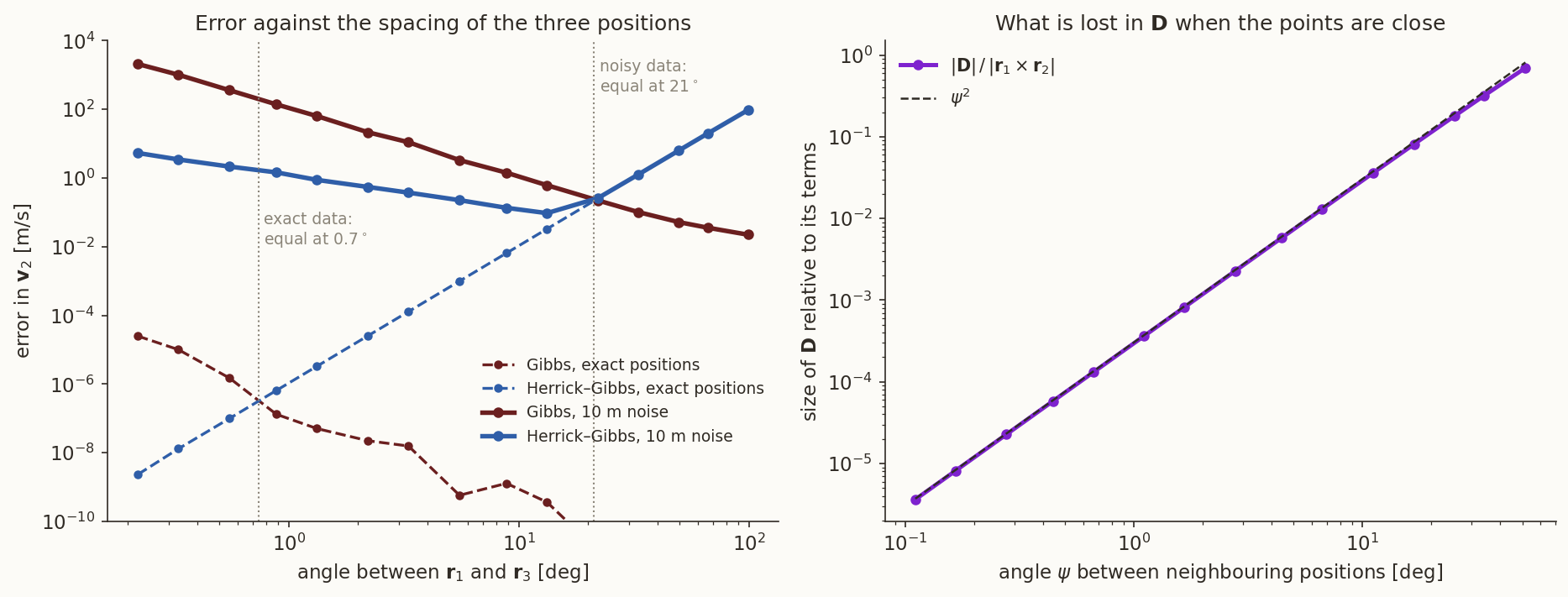
Gibbs’s formula is exact, so one might expect it to be best. It is not, when the three positions are close together. Figure 3 (left) shows why this happens and what to do instead.
3.1 Why Gibbs fails
Look at \(\mathbf D=\mathbf r_1\times\mathbf r_2+\mathbf r_2\times\mathbf r_3+\mathbf r_3\times\mathbf r_1\). On a circular orbit of radius \(r\) with neighbouring positions \(\psi\) apart, each of the first two terms has length \(r^2\sin\psi\) and the third, pointing the other way, \(r^2\sin2\psi\), so
\[ D=r^{2}\,(2\sin\psi-\sin2\psi)\approx r^{2}\psi^{3},\qquad\text{while each term is}\approx r^{2}\psi . \]
The sum is \(\psi^{2}\) times smaller than its terms: three numbers of size \(r^2\psi\) that nearly cancel. A position error \(\delta r/r\) shows up in \(D\) as a relative error of about \((\delta r/r)/\psi^2\). At \(1.1^\circ\) between \(\mathbf r_1\) and \(\mathbf r_3\) (\(\psi=0.55^\circ\)), \(\lVert\mathbf D\rVert/\lVert\mathbf r_1\times\mathbf r_2\rVert=9\times10^{-5}\), and a \(1\) m rounding of positions \(7600\) km from the centre (\(1.3\times10^{-7}\)) is magnified about ten thousand times. The same cancellation sits in \(\mathbf N\) and \(\mathbf S\). Figure 3 (right) shows that the ratio is indeed \(\psi^2\) over the whole range, for the orbit of the example.
3.2 The idea of Herrick–Gibbs
When the points are close, the time spacing is short, and the velocity can be had by a Taylor series in time instead of the conic. The new ingredient is the times \(t_1,t_2,t_3\). The derivation has two steps.
Step 1: interpolation. Expand the positions about \(t_2\), \[ \mathbf r_i-\mathbf r_2=\tau_i\mathbf v_2+\tfrac12\tau_i^2\mathbf a_2+\tfrac16\tau_i^3\dot{\mathbf a}_2+\tfrac1{24}\tau_i^4\ddot{\mathbf a}_2+O(\tau^5),\qquad i=1,3 . \] Eliminate the acceleration \(\mathbf a_2\) (which we have not got yet) by forming \(\tau_3^2(\mathbf r_1-\mathbf r_2)-\tau_1^2(\mathbf r_3-\mathbf r_2)\); the terms in \(\tau_1^2\tau_3^2\) cancel, and \[ \begin{aligned} \mathbf v_2&=\frac{\tau_3^{2}(\mathbf r_1-\mathbf r_2)-\tau_1^{2}(\mathbf r_3-\mathbf r_2)}{\tau_1\tau_3(\tau_3-\tau_1)}\\ &\quad+\frac{\tau_1\tau_3}{6}\,\dot{\mathbf a}_2+\frac{\tau_1\tau_3(\tau_1+\tau_3)}{24}\,\ddot{\mathbf a}_2+O(\tau^{4}). \end{aligned} \tag{9}\] The first term is the velocity of the parabola through the three points, and the others are what it misses.
Step 2: the missing terms are known. The jerk \(\dot{\mathbf a}_2\) and the snap \(\ddot{\mathbf a}_2\) are derivatives of the acceleration, and the acceleration is a function of position alone, \(\mathbf a_i=-\mu\mathbf r_i/r_i^3\), so we know \(\mathbf a_1,\mathbf a_2,\mathbf a_3\) from the three positions. Expand them about \(t_2\) too, \(\mathbf a_i=\mathbf a_2+\tau_i\dot{\mathbf a}_2+\tfrac12\tau_i^2\ddot{\mathbf a}_2+\dots\), and form \(\tau_3\mathbf a_1-(\tau_1+\tau_3)\mathbf a_2+\tau_1\mathbf a_3\): the terms in \(\mathbf a_2\) cancel, and \[ \tau_3\mathbf a_1-(\tau_1+\tau_3)\mathbf a_2+\tau_1\mathbf a_3 =2\tau_1\tau_3\,\dot{\mathbf a}_2+\tfrac12\tau_1\tau_3(\tau_1+\tau_3)\,\ddot{\mathbf a}_2+O(\tau^5). \] One twelfth of this is exactly the two correction terms of Equation 9. So
\[ \boxed{\begin{aligned} \mathbf v_2&=\frac{\tau_3^{2}(\mathbf r_1-\mathbf r_2)-\tau_1^{2}(\mathbf r_3-\mathbf r_2)}{\tau_1\tau_3(\tau_3-\tau_1)}\\ &\quad-\frac{\mu}{12}\left[\tau_3\frac{\mathbf r_1}{r_1^{3}}-(\tau_1+\tau_3)\frac{\mathbf r_2}{r_2^{3}}+\tau_1\frac{\mathbf r_3}{r_3^{3}}\right] \end{aligned}} \tag{10}\]
with an error \(O(\tau^4)\): for equal spacing, \(+\tfrac{7}{360}\tau^{4}\,\mathbf r^{(5)}_2\). (The verify script confirms the whole chain symbolically: the combination reproduces the derivative of any polynomial history of degree \(\le4\) exactly, the interpolation alone is exact only through degree \(2\), and the leading error is the one quoted.) The conic never appeared: Equation 10 is a statement about smooth curves, and gravity entered only through \(\mathbf a=-\mu\mathbf r/r^3\).
History. The combination of a Taylor series in the times with the gravitational acceleration at the three points is usually called the Herrick–Gibbs method in the textbooks (Vallado 2013), a close-spaced companion of Gibbs’s method.
3.3 Example 2: three positions \(10\) s apart
The scenario at \(t=-10,0,+10\) s, positions rounded to \(1\) m: \(\mathbf r_1=(4620.412,\,-5595.624,\,2245.568)\), \(\mathbf r_2=(4656.838,\,-5551.747,\,2291.717)\), \(\mathbf r_3=(4692.842,\,-5507.365,\,2337.657)\) km. The angle between \(\mathbf r_1\) and \(\mathbf r_3\) is \(1.10^\circ\).
| \(\mathbf v_2\) [km/s] | error [m/s] | |
|---|---|---|
| truth | \((3.621537,\ 4.413025,\ 4.604554)\) | |
| Gibbs, Equation 8 | \((3.620416,\ 4.411655,\ 4.603080)\) | \(2.30\) |
| Herrick–Gibbs, Equation 10 | \((3.621544,\ 4.413030,\ 4.604514)\) | \(0.040\) |
With exact positions both are good to \(10^{-6}\) m/s; the difference is entirely the metre of rounding, amplified by Gibbs’s cancellation and not by Herrick–Gibbs’s.
3.4 Which one when?
Figure 3 shows two regimes. With exact data, Gibbs is better for every spacing larger than \(0.74^\circ\) (below that, double precision itself starts to be exhausted), and Herrick–Gibbs’s \(\tau^4\) truncation error takes over beyond. With \(10\) m of noise per coordinate, which is the realistic case, the curves cross at \(21^\circ\): below that Herrick–Gibbs is better, above it Gibbs. Herrick–Gibbs’s best error is \(0.09\) m/s at about \(13^\circ\), and Gibbs’s error keeps decreasing as the points spread out (\(0.10\) m/s at \(33^\circ\), \(0.02\) m/s at \(99^\circ\)) because noise matters less for widely separated points. The rule of thumb is therefore Herrick–Gibbs for points within a few tens of degrees of each other, Gibbs beyond, and the noise level decides the dividing line.
4 Two positions and the time: Lambert
If the time of flight \(\Delta t\) between two position fixes is known, the velocity follows from Lambert’s problem: find the Kepler orbit that joins \(\mathbf r_1\) to \(\mathbf r_3\) in time \(\Delta t\). The Lambert note formulates and solves it, and the universal-variables note gives the solver used here; as an orbit-determination method it needs no new theory, only a change of viewpoint: the solver returns \(\mathbf v_1\) and \(\mathbf v_3\), and the state at any other time is a propagation away.
Example 3. Take the outer two positions of Example 1, \(\mathbf r_1\) and \(\mathbf r_3\) (\(t=\mp300\) s, rounded to \(1\) m), and \(\Delta t=600\) s. The transfer angle is \(33.117^\circ\) and the universal-variable equation converges to \(z=0.3184\). The velocities returned differ from the true ones by \(0.0011\) m/s at \(\mathbf r_1\) and \(0.0010\) m/s at \(\mathbf r_3\); propagating \(\mathbf v_1\) forward by \(300\) s gives the state at \(t=0\) to \(0.33\) m and \(0.0011\) m/s. That is better than the three-position Gibbs result of Example 1, though it used one position less: the time was information.
With noise the gap widens. For \(10\) m of noise per coordinate, the median velocity error at \(t=0\) is \(0.037\) m/s from Lambert (two positions, propagated) against \(0.11\) m/s from Gibbs (three positions) in \(400\) trials. The price is that the clock must be right: a timing error \(\delta t\) between the two fixes moves the satellite along its track by \(v\,\delta t\), \(7.3\) m for a millisecond, and Lambert’s method reads it as a position error. (It also has to be told the direction of motion and the number of complete revolutions; for a satellite tracked through one pass, zero.)
Run the universal-variable Lambert solver on the rounded positions \(\mathbf r_1,\mathbf r_3\) of Example 1 with \(\Delta t=600\) s, then propagate to \(t=0\) and compare with the true state.
What you should find
\(\mathbf v_1=(4.748842,\ 2.704460,\ 5.041449)\) km/s against the truth \((4.748841,\ 2.704460,\ 5.041448)\); at \(t=0\) the error is \(0.33\) m in position and \(1.1\times10^{-3}\) m/s in velocity.5 Angles only: the problem
A telescope gives two numbers per epoch, the right ascension and declination of the line of sight. With the station’s position \(\mathbf R_i\) at the epoch (the site vector of the topocentric note, turned by the sidereal angle), the satellite is somewhere along the line of sight,
\[ \mathbf r_i=\mathbf R_i+\rho_i\,\mathbf L_i,\qquad \mathbf L_i=\begin{bmatrix}\cos\delta_i\cos\alpha_i\\ \cos\delta_i\sin\alpha_i\\ \sin\delta_i\end{bmatrix}, \tag{11}\]
and the one thing the telescope cannot say is how far: the range \(\rho_i\). Three epochs leave three unknown ranges. If they were known, Equation 11 would give three positions and Gibbs’s method the velocity, so the whole problem is to find \(\rho_1,\rho_2,\rho_3\). The equations that determine them come from the dynamics: the three positions must be coplanar with the Earth’s centre (one condition), and the intervals between them must agree with Kepler’s equation (two more). The two classical methods use that information in different ways.
- Laplace’s method (Section 6) is local: it differentiates the observed direction in time and uses the equation of motion at the middle epoch.
- Gauss’s method (Section 7) is global: it writes the three positions as combinations of one another through the Lagrange coefficients, which is an exact statement about Kepler motion.
Both end in the same polynomial of degree eight for \(r_2\). A point to keep in mind throughout: the range is not measured; it is inferred from the curvature of the line-of-sight track on the sky. A small curvature is a small signal, and Section 8 is about what that does.
6 Laplace’s method
History: Laplace. Laplace’s method, from his memoir on the orbits of comets (Laplace 1784), differentiates the observed direction of a comet and uses Newton’s law at one instant. It needs the derivatives of the observed direction, which is why it asks for closely spaced, accurate observations. Gauss’s method, published in 1809 (Gauss 1809), takes no derivatives of the observations.
6.1 Derivatives of the line of sight
From the three directions we construct \(\mathbf L_2\), \(\dot{\mathbf L}_2\) and \(\ddot{\mathbf L}_2\) by fitting a parabola, \(\mathbf L(t)\approx\mathbf L_2+\dot{\mathbf L}_2\,(t-t_2)+\tfrac12\ddot{\mathbf L}_2\,(t-t_2)^2\), through the three observations. Requiring it to pass through \(\mathbf L_1\) at \(t=\tau_1\) and through \(\mathbf L_3\) at \(t=\tau_3\) gives two linear equations for \(\dot{\mathbf L}_2\) and \(\ddot{\mathbf L}_2\) whose solution is
\[ \begin{aligned} \dot{\mathbf L}_2&=\frac{\tau_3^{2}(\mathbf L_1-\mathbf L_2)-\tau_1^{2}(\mathbf L_3-\mathbf L_2)}{\tau_1\tau_3(\tau_3-\tau_1)},\\ \ddot{\mathbf L}_2&=\frac{2\,\bigl[\tau_3(\mathbf L_1-\mathbf L_2)-\tau_1(\mathbf L_3-\mathbf L_2)\bigr]}{\tau_1\tau_3(\tau_1-\tau_3)} . \end{aligned} \tag{12}\]
For equal spacing \(h\) these are the familiar central differences \((\mathbf L_3-\mathbf L_1)/2h\) and \((\mathbf L_1-2\mathbf L_2+\mathbf L_3)/h^2\). The first is the same quadratic interpolation as in Equation 9; the price is the error of the interpolation, which grows with the arc as \(h^2\) and is the weak point of the method.
6.2 Eliminating the range rates
Differentiate \(\mathbf r=\mathbf R+\rho\mathbf L\) twice and set \(\ddot{\mathbf r}=-\mu\mathbf r/r^3=-\mu(\mathbf R+\rho\mathbf L)/r^3\): \[ \ddot{\mathbf R}+\ddot\rho\,\mathbf L+2\dot\rho\,\dot{\mathbf L}+\rho\,\ddot{\mathbf L}=-\frac{\mu}{r^{3}}\,(\mathbf R+\rho\mathbf L). \] Collect the unknown ranges on the left, \[ \ddot\rho\,\mathbf L+2\dot\rho\,\dot{\mathbf L}+\rho\Bigl(\ddot{\mathbf L}+\frac{\mu}{r^{3}}\mathbf L\Bigr)=-\Bigl(\ddot{\mathbf R}+\frac{\mu}{r^{3}}\mathbf R\Bigr). \qquad\qquad (**) \] This is a vector equation (three scalar ones) for the three unknowns \(\rho,\dot\rho,\ddot\rho\), with the unknown \(r\) in the coefficients. The trick is to dot it with a vector that is perpendicular to both \(\mathbf L\) and \(\dot{\mathbf L}\), which kills the first two terms: \(\mathbf n=\mathbf L\times\dot{\mathbf L}\). Then only \(\rho\) survives on the left, because \(\mathbf L\cdot\mathbf n=0\) and \(\ddot{\mathbf L}\cdot\mathbf n=D\), where
\[ D=\mathbf L\cdot(\dot{\mathbf L}\times\ddot{\mathbf L})=\ddot{\mathbf L}\cdot(\mathbf L\times\dot{\mathbf L}) \]
(the same triple product, cyclically permuted). Dotting \((**)\) with \(\mathbf n\) gives \(\rho\,D=-\ddot{\mathbf R}\cdot\mathbf n-\mu\,(\mathbf R\cdot\mathbf n)/r^3\), that is
\[ \begin{aligned} \rho&=A+\frac{B}{r^{3}},\\ A&=-\frac{D_1}{D},\quad B=-\frac{\mu D_2}{D},\quad D_1=\ddot{\mathbf R}\cdot\mathbf n,\quad D_2=\mathbf R\cdot\mathbf n . \end{aligned} \tag{13}\]
All quantities are at the middle epoch, and \(A,B\) are known from the data. Equation 13 is the first of two relations between the range \(\rho\) and the unknown distance \(r\).
6.3 The second relation and the polynomial of degree eight
The second relation is pure geometry: \(r^2=\lVert\mathbf R+\rho\mathbf L\rVert^2\), so, with \(C=\mathbf L\cdot\mathbf R\),
\[ r^{2}=\rho^{2}+2C\rho+R^{2},\qquad\text{i.e.}\qquad \rho=-C+\sqrt{r^{2}-R^{2}+C^{2}} . \tag{14}\]
(The root with the minus sign is negative whenever \(C>0\), that is whenever the satellite is above the horizon, and would put the satellite behind the station.) Substituting Equation 13 into the first form and multiplying by \(r^6\):
\[ r^{8}-\bigl(A^{2}+2AC+R^{2}\bigr)\,r^{6}-2B\,(A+C)\,r^{3}-B^{2}=0 . \tag{15}\]
It is a polynomial of degree eight in \(r\) (because \(\rho\) is a function of \(r^3\) and the relation is quadratic in \(\rho\)). We want its positive real root.
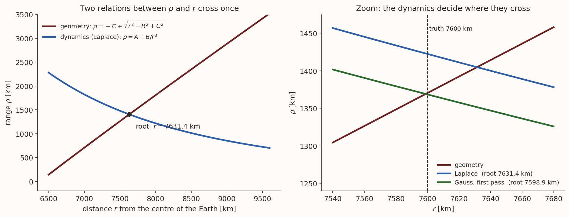
Which root? Descartes’s rule of signs counts the sign changes of the coefficients: the leading one is \(+1\), the coefficient of \(r^6\) is \(-(A^2+2AC+R^2)=-\lVert\mathbf R+A\mathbf L\rVert^2\le0\) and that of \(r^0\) is \(-B^2\le0\). If the coefficient \(-2B(A+C)\) of \(r^3\) is also negative or zero, there is exactly one sign change and so exactly one positive root. A graphical argument says the same (Figure 4, left). The function Equation 13 is decreasing in \(r\) when \(B>0\), while the geometric Equation 14 is increasing, so they cross at most once. In every example of this note, for every arc, \(B>0\) and the root is unique. (When \(B<0\) the argument fails, the sign of \(B\) depending on the geometry, and Descartes’s rule allows up to three positive roots. One then keeps the roots with \(\rho>0\) and chooses among them with whatever else is known about the object, for instance that it is above the surface of the Earth. The verify script lists every positive root of every example.)
6.4 The range rate and the state
With \(r\) known, \(\rho\) comes from Equation 13. For \(\dot\rho\), dot \((**)\) with \(\mathbf m=\mathbf L\times\ddot{\mathbf L}\), which is perpendicular to \(\mathbf L\) and \(\ddot{\mathbf L}\), so that both the \(\ddot\rho\) term and the \(\rho\) term vanish (the \(\rho\) term is \(\rho\,(\ddot{\mathbf L}+\mu\mathbf L/r^3)\cdot\mathbf m=0\)). What is left is \(2\dot\rho\,\dot{\mathbf L}\cdot\mathbf m=-(\ddot{\mathbf R}+\mu\mathbf R/r^3)\cdot\mathbf m\), and \(\dot{\mathbf L}\cdot(\mathbf L\times\ddot{\mathbf L})=-D\), so
\[ \begin{aligned} \dot\rho&=\frac{\bigl(\ddot{\mathbf R}+\mu\mathbf R/r^{3}\bigr)\cdot\mathbf m}{2D},\\ \mathbf r_2&=\mathbf R_2+\rho\,\mathbf L_2,\qquad \mathbf v_2=\dot{\mathbf R}_2+\dot\rho\,\mathbf L_2+\rho\,\dot{\mathbf L}_2 . \end{aligned} \tag{16}\]
The last is the derivative of \(\mathbf r=\mathbf R+\rho\mathbf L\).
6.5 Example 4: three directions \(60\) s apart
A telescope has measured, at \(t=-60,0,+60\) s, the topocentric right ascension and declination (rounded to \(10^{-6}\) degrees, which is \(3.6\) mas):
| \(t\) [s] | \(\alpha\) [deg] | \(\delta\) [deg] | \(\mathbf R\) [km] |
|---|---|---|---|
| \(-60\) | \(278.718649\) | \(21.409699\) | \((4235.280,\ -4524.291,\ 1502.908)\) |
| \(0\) | \(291.012940\) | \(35.143647\) | \((4255.034,\ -4505.718,\ 1502.908)\) |
| \(+60\) | \(306.798619\) | \(47.050460\) | \((4274.707,\ -4487.058,\ 1502.908)\) |
The station’s velocity and acceleration at \(t=0\) are \(\dot{\mathbf R}=(0.328562,\ 0.310282,\ 0)\) km/s and \(\ddot{\mathbf R}=(-2.2626,\ 2.3959,\ 0)\times10^{-5}\) km/s\(^2\). The unit vectors are \(\mathbf L_1=(0.141122,\,-0.920236,\,0.365034)\), \(\mathbf L_2=(0.293214,\,-0.763333,\,0.575628)\), \(\mathbf L_3=(0.408134,\,-0.545591,\,0.731954)\), and Equation 12 gives
\[ \begin{aligned} \dot{\mathbf L}_2&=(2.2251,\ 3.1220,\ 3.0577)\times10^{-3}\ \text{s}^{-1},\\ \ddot{\mathbf L}_2&=(-1.0325,\ 1.6900,\ -1.5075)\times10^{-5}\ \text{s}^{-2}. \end{aligned} \]
Then \(D=9.7466\times10^{-9}\) s\(^{-3}\), \(D_1=1.0268\times10^{-7}\) km s\(^{-3}\), \(D_2=-15.381\) km/s, so
\[ A=-10.535\ \text{km},\qquad B=6.2903\times10^{14}\ \text{km}^{4},\qquad C=5552.115\ \text{km}, \]
and the polynomial Equation 15 has the coefficients \(-A^2-2AC-R^2=-4.0549\times10^{7}\) km\(^2\), \(-2B(A+C)=-6.9717\times10^{18}\) km\(^5\) and \(-B^2=-3.9568\times10^{29}\) km\(^8\). The coefficient of \(r^3\) is negative, so there is one positive root (the other seven are one negative real and three complex-conjugate pairs): \[ r=7631.402\ \text{km}. \] Then \(\rho=1404.806\) km, \(\dot\rho=0.45780\) km/s, and \[ \begin{aligned} \mathbf r_2&=(4666.943,\ -5578.052,\ 2311.554)\ \text{km},\\ \mathbf v_2&=(3.58862,\ 4.34669,\ 4.55894)\ \text{km/s}. \end{aligned} \] The truth is \(\rho=1370.344\) km, \(\dot\rho=0.48430\) km/s, \(r=7600\) km. The method has returned the state to \(34.5\) km and \(87\) m/s, and the elements \(a=7679\) km, \(e=0.0553\) (true \(7800\), \(0.0583\)) are rough. That error is not noise (the data are rounded to \(3.6\) mas): it is the error of fitting a parabola to a line of sight that moves \(34^\circ\) across the sky. Replace the interpolated derivatives by the exact ones, obtained from a high-order finite difference of the true line of sight, and the algebra above returns the truth to \(4\times10^{-7}\) km. The error is \(1.0\) km for the same method with \(\pm10\) s, \(34\) km for \(\pm60\) s, \(128\) km for \(\pm120\) s and \(408\) km for \(\pm240\) s: it grows roughly as the square of the arc.
At \(r=7600\) km, what range does the geometry Equation 14 give, and what range does the dynamics Equation 13 give? Which way must \(r\) move to make them agree?
What you should find
Geometry: \(\rho=1370.3\) km (that is the true range, since \(r=7600\) km is the true distance). Dynamics: \(\rho=A+B/r^3=1422.4\) km, \(52\) km too large; the dynamical curve falls with \(r\) and the geometric one rises, so \(r\) must increase, to \(7631.4\) km, where both give \(1404.8\) km.Why can’t one simply shorten the arc until the parabola fits perfectly?
Answer
Because the signal that carries the range shrinks even faster than the interpolation error: the range is inferred from the curvature of the line-of-sight track, which is proportional to \(h^2\), and the measurement noise does not shrink. With the arc \(\pm10\) s the interpolation error is \(1\) km (noise-free) but a \(2''\) noise makes the error \(77\) km. Section 8 has the numbers.7 Gauss’s method
History: Gauss and Ceres. Giuseppe Piazzi, observing at Palermo, found the small planet Ceres on 1 January 1801 and followed it for 41 days before it disappeared in the glare of the Sun. The arc was short, and the problem of predicting where to look next, from a few observations, was set to the mathematicians. The young Gauss solved it, and Ceres was found again at the end of 1801, close to the predicted position (Zach and Olbers are credited with the recovery; Olbers observed it in Bremen on the last day of the year). Gauss set out the method in the Theoria motus (Gauss 1809). The form given here is the modern textbook form (for example (Curtis 2014)) with the Lagrange coefficients, organised differently from Gauss’s own account but resting on the same idea.
7.1 From the Lagrange coefficients to a relation between the positions
Kepler motion carries the state at \(t_2\) to the state at any other time by the Lagrange coefficients (the universal-variables note): \(\mathbf r_1=F_1\mathbf r_2+G_1\mathbf v_2\) and \(\mathbf r_3=F_3\mathbf r_2+G_3\mathbf v_2\), where the coefficients are those of the intervals \(\tau_1\) and \(\tau_3\). These are two equations for the unknowns \(\mathbf r_2\) and \(\mathbf v_2\) in terms of \(\mathbf r_1\) and \(\mathbf r_3\). Eliminating \(\mathbf v_2\) (multiply the first by \(G_3\), the second by \(G_1\), subtract) gives \(G_3\mathbf r_1-G_1\mathbf r_3=(F_1G_3-F_3G_1)\,\mathbf r_2\); eliminating \(\mathbf r_2\) in the same way gives \(F_1\mathbf r_3-F_3\mathbf r_1=(F_1G_3-F_3G_1)\,\mathbf v_2\). So
\[ \begin{aligned} \mathbf r_2&=c_1\,\mathbf r_1+c_3\,\mathbf r_3,\qquad \mathbf v_2=\frac{F_1\,\mathbf r_3-F_3\,\mathbf r_1}{F_1G_3-F_3G_1},\\ c_1&=\frac{G_3}{F_1G_3-F_3G_1},\qquad c_3=-\frac{G_1}{F_1G_3-F_3G_1}. \end{aligned} \tag{17}\]
The first says that the middle position is a combination of the outer two, with weights \(c_1,c_3\) (both close to \(\tfrac12\) for equal spacing, as the middle point is roughly the midpoint of the chord). The weights depend on the orbit only through \(F\) and \(G\).
7.2 The three ranges
Put \(\mathbf r_i=\mathbf R_i+\rho_i\mathbf L_i\) into \(\mathbf r_2=c_1\mathbf r_1+c_3\mathbf r_3\) and collect the unknown ranges on the left:
\[ c_1\rho_1\,\mathbf L_1-\rho_2\,\mathbf L_2+c_3\rho_3\,\mathbf L_3=-c_1\mathbf R_1+\mathbf R_2-c_3\mathbf R_3 . \tag{18}\]
Given \(c_1\) and \(c_3\) this is a linear system for \(\rho_1,\rho_2,\rho_3\), and it is solved by the same trick as before, dotting with the cross product of two of the \(\mathbf L\)’s to kill the other two terms. Let
\[ \begin{aligned} \mathbf p_1&=\mathbf L_2\times\mathbf L_3,\quad \mathbf p_2=\mathbf L_1\times\mathbf L_3,\quad \mathbf p_3=\mathbf L_1\times\mathbf L_2,\\ D_0&=\mathbf L_1\cdot\mathbf p_1,\qquad D_{ij}=\mathbf R_i\cdot\mathbf p_j . \end{aligned} \]
Then \(\mathbf L_1\cdot\mathbf p_1=D_0\), \(\mathbf L_2\cdot\mathbf p_2=\mathbf L_2\cdot(\mathbf L_1\times\mathbf L_3)=-D_0\), \(\mathbf L_3\cdot\mathbf p_3=D_0\), and each product with the “wrong” \(\mathbf L\) is zero. Dotting Equation 18 with \(\mathbf p_1,\mathbf p_2,\mathbf p_3\) in turn:
\[ \begin{aligned} \rho_1&=\frac1{D_0}\Bigl(-D_{11}+\frac{D_{21}}{c_1}-\frac{c_3}{c_1}D_{31}\Bigr),\\ \rho_2&=\frac1{D_0}\bigl(-c_1D_{12}+D_{22}-c_3D_{32}\bigr),\\ \rho_3&=\frac1{D_0}\Bigl(-\frac{c_1}{c_3}D_{13}+\frac{D_{23}}{c_3}-D_{33}\Bigr). \end{aligned} \tag{19}\]
(\(D_0\) is the triple product of the three lines of sight; it is the determinant of the system, and it will matter in Section 8.) So everything hinges on \(c_1\) and \(c_3\), which depend on the orbit through \(F\) and \(G\), which depend on the unknown state.
7.3 The first pass: series for \(F\) and \(G\)
Gauss’s way out is to expand \(F\) and \(G\) in the time interval and keep the first terms. With \(\mathbf a=-\mu\mathbf r/r^3\), the Taylor series of \(\mathbf r(t_2+\tau)\) is \(\mathbf r_2+\tau\mathbf v_2-\tfrac12\tau^2\mu\mathbf r_2/r_2^3+\dots\), so, with \(u=\mu/r_2^3\),
\[ F\approx1-\frac{u\,\tau^{2}}{2},\qquad G\approx\tau-\frac{u\,\tau^{3}}{6} \]
(the next terms carry the radial velocity of the satellite and are smaller; here \(v_r/r\approx5\times10^{-5}\) s\(^{-1}\)). The determinant of Equation 17 is then, to first order in \(u\),
\[ F_1G_3-F_3G_1\approx\tau_3-\tau_1-u\Bigl[\frac{\tau_3^{3}}6-\frac{\tau_1^{3}}6+\frac{\tau_1^{2}\tau_3}2-\frac{\tau_3^{2}\tau_1}2\Bigr]=\tau-\frac{u\,\tau^{3}}6, \]
because the bracket is \((\tau_3-\tau_1)^3/6\). (Expand \((\tau_3-\tau_1)^3\) to check.) Using this and \(G_3\approx\tau_3(1-u\tau_3^2/6)\), \(G_1\approx\tau_1(1-u\tau_1^2/6)\), we get from Equation 17, again to first order in \(u\) (use \(1/(1-x)\approx1+x\)),
\[ c_1\approx\frac{\tau_3}{\tau}\Bigl[1+\frac u6\bigl(\tau^{2}-\tau_3^{2}\bigr)\Bigr],\qquad c_3\approx-\frac{\tau_1}{\tau}\Bigl[1+\frac u6\bigl(\tau^{2}-\tau_1^{2}\bigr)\Bigr]. \tag{20}\]
Put this into the middle line of Equation 19. The terms free of \(u\) and those proportional to \(u=\mu/r_2^3\) separate:
\[ \begin{aligned} \rho_2&=A+\frac{\mu B}{r_2^{3}},\\ A&=\frac1{D_0}\Bigl(-\frac{\tau_3}{\tau}D_{12}+D_{22}+\frac{\tau_1}{\tau}D_{32}\Bigr),\\ B&=\frac1{6D_0}\Bigl[\frac{\tau_3}{\tau}\bigl(\tau_3^{2}-\tau^{2}\bigr)D_{12}+\frac{\tau_1}{\tau}\bigl(\tau^{2}-\tau_1^{2}\bigr)D_{32}\Bigr]. \end{aligned} \tag{21}\]
This is the same form as Equation 13, and it combines with the same geometric relation Equation 14 (\(E=\mathbf R_2\cdot\mathbf L_2\) is the \(C\) of that equation) to the same polynomial,
\[ r_2^{8}-\bigl(A^{2}+2AE+R_2^{2}\bigr)\,r_2^{6}-2\mu B\,(A+E)\,r_2^{3}-\mu^{2}B^{2}=0 . \tag{22}\]
The root story is as for Laplace (Figure 4, right, shows both curves). With the root \(r_2\): \(u=\mu/r_2^3\), then \(c_1,c_3\) from Equation 20, the ranges from Equation 19, the three positions from Equation 11, and \(\mathbf v_2\) from Equation 17.
7.4 Iterating
This first pass is accurate only to the first order in \(u\tau^2\), so its error grows as \(h^2\) (below). Here is the improvement that makes Gauss’s method the better method. Having a state \((\mathbf r_2,\mathbf v_2)\), compute the exact Lagrange coefficients by universal variables (the universal-variables note) rather than the series; recompute \(c_1,c_3\) from Equation 17, the ranges from Equation 19, the three positions, and \(\mathbf v_2\) from Equation 17; and repeat until the ranges stop changing. At convergence the three positions and the velocity satisfy \(\mathbf r_i=F_i\mathbf r_2+G_i\mathbf v_2\) exactly, with the exact \(F_i,G_i\) of that very state: they lie on a Kepler orbit, and each lies on its observed line of sight. For noise-free data that orbit is the true one.
7.5 Example 5: the same data
Use the data of Example 4. \(D_0=2.1053\times10^{-3}\), and the matrix of \(D_{ij}=\mathbf R_i\cdot\mathbf p_j\) (km) is
\[ \begin{bmatrix}-900.350&-1767.223&-936.454\\-904.805&-1775.746&-940.934\\-909.240&-1784.226&-945.392\end{bmatrix}. \]
Equation 21 gives \(A=-10.114\) km and \(B=1.5182\times10^{9}\) km s\(^2\), and Equation 22 has the coefficients \(-4.0553\times10^{7}\) km\(^2\), \(-6.7077\times10^{18}\) km\(^5\) and \(-3.6623\times10^{29}\) km\(^8\): again one positive root, \(r_2=7598.869\) km. Then \(c_1=c_3=0.5008176\), \(\rho=(1392.943,\ 1369.103,\ 1448.501)\) km, and the first pass gives
\[ \begin{aligned} \mathbf r_2&=(4656.474,\ -5550.799,\ 2291.002)\ \text{km},\\ \mathbf v_2&=(3.61893,\ 4.40890,\ 4.60054)\ \text{km/s}, \end{aligned} \]
with an error of \(1.24\) km and \(6.3\) m/s: against \(34\) km and \(87\) m/s for Laplace on the same data. The iteration reduces it:
| iteration | \(\rho_2\) [km] | \(\lvert\Delta\mathbf r_2\rvert\) [km] | \(\lvert\Delta\mathbf v_2\rvert\) [m/s] |
|---|---|---|---|
| 0 (first pass) | \(1369.1027\) | \(1.2416\) | \(6.315\) |
| 1 | \(1370.9636\) | \(0.6193\) | \(3.156\) |
| 2 | \(1370.0353\) | \(0.3090\) | \(1.575\) |
| 4 | \(1370.2674\) | \(0.0770\) | \(0.392\) |
| 8 | \(1370.3395\) | \(0.0049\) | \(0.025\) |
| 12 | \(1370.3439\) | \(0.0004\) | \(0.002\) |
True \(\rho_2=1370.3443\) km. The error is halved at every iteration (Figure 5) until it reaches the floor set by the rounding of the angles, about \(0.1\) m, and the range alternates between too large and too small. After \(32\) iterations the ranges stop changing at the tolerance \(10^{-12}\); the position error is \(0.12\) m and the velocity error \(0.7\) mm/s, which is the effect of rounding the angles to \(3.6\) mas. The elements are \(a=7799.998\) km, \(e=0.05830\), \(i=43.0811^\circ\), \(\Omega=290.2235^\circ\), \(\omega=319.2685^\circ\), \(f=66.9295^\circ\): the true orbit.
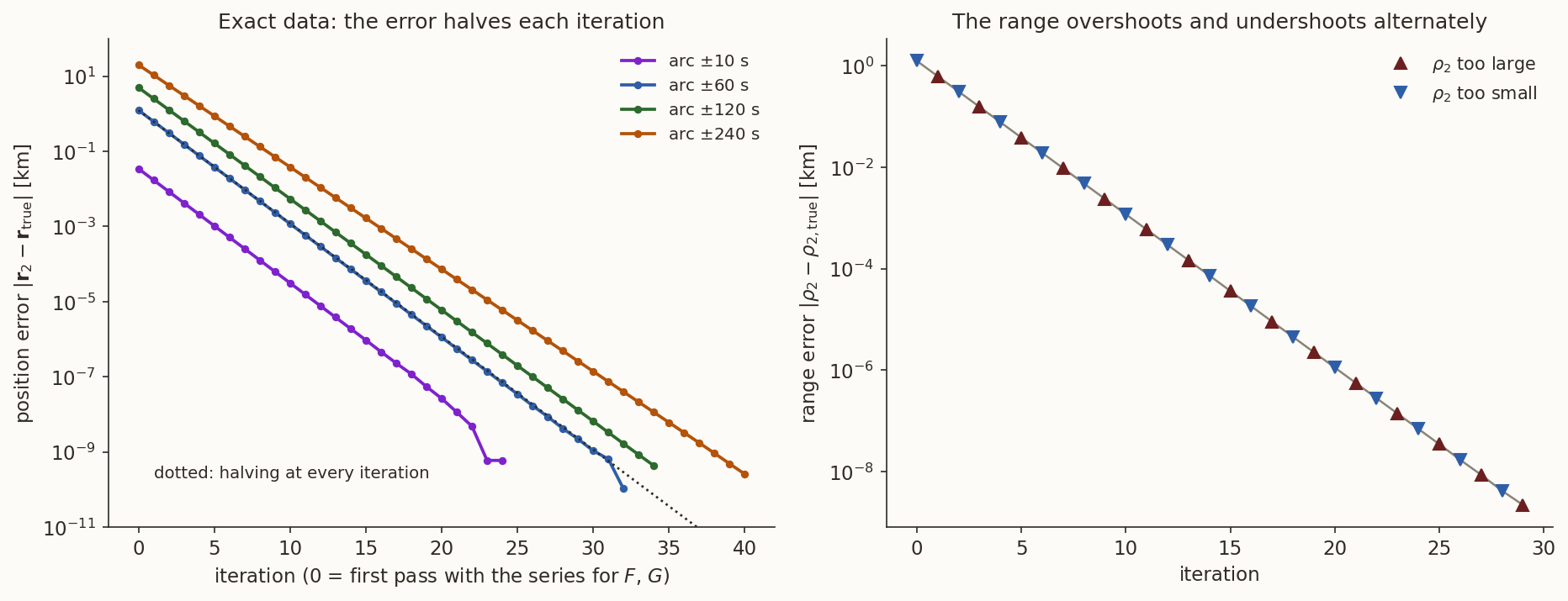
For the data of Example 5, compute the exact coefficients from the true state, \(F_1,G_1,F_3,G_3\) over \(\mp60\) s, and compare \(c_1,c_3\) with the series of Equation 20.
What you should find
Exact: \(c_1=0.5008196\), \(c_3=0.5008171\) (they differ, since the true orbit is not symmetric about \(t_2\)); series: both \(0.5008172\). The two agree to about \(2\times10^{-6}\), and the first-pass error of Example 5 comes from differences of that size, which Equation 19 multiplies by numbers of order \(10^3\) km and divides by \(D_0=2\times10^{-3}\).8 How good is it? Noise, arc and geometry
All results so far were for data that are exact or rounded to \(3.6\) mas. A real telescope measures to about \(1''\) to \(2''\), and the radars that give positions to metres or tens of metres are common. We add Gaussian noise of \(2''\) (on \(\alpha\cos\delta\) and on \(\delta\), independently; \(13\) m across the line of sight at the \(1370\) km range of the middle epoch) to the lines of sight, run each method on 300 noisy sets for each arc \(\pm h\) and record the position error at \(t=0\): the median and the central 68 % (Figure 6; the numbers are reproducible, with fixed seeds).
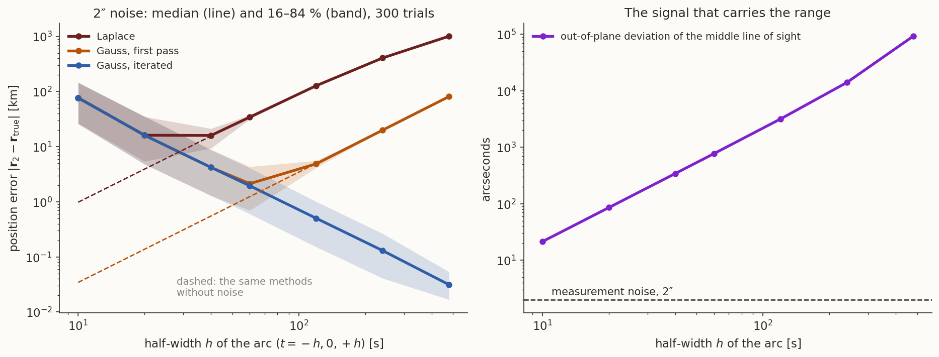
| \(h\) [s] | \(D_0\) | out of plane | Laplace [km] | Gauss, first pass [km] | Gauss, iterated [km] |
|---|---|---|---|---|---|
| \(10\) | \(1.0\times10^{-5}\) | \(21''\) | \(77\) | \(77\) | \(77\) |
| \(20\) | \(8.3\times10^{-5}\) | \(85''\) | \(16\) | \(16\) | \(16\) |
| \(40\) | \(6.5\times10^{-4}\) | \(342''\) | \(16\) | \(4.2\) | \(4.2\) |
| \(60\) | \(2.1\times10^{-3}\) | \(772''\) | \(34\) | \(2.1\) | \(2.0\) |
| \(120\) | \(1.4\times10^{-2}\) | \(3164''\) | \(128\) | \(4.9\) | \(0.50\) |
| \(240\) | \(6.4\times10^{-2}\) | \(14\,016''\) | \(408\) | \(20\) | \(0.13\) |
| \(480\) | \(0.19\) | \(92\,769''\) | \(1012\) | \(81\) | \(0.031\) |
Three things are visible.
- Short arcs are noise-limited. For \(h\le20\) s all three methods give the same error, set by the noise, and it falls about four-fold each time the arc doubles: the error in the range goes as \(\sigma/h^{2}\). The reason is in the right panel of the figure: the range is carried by the curvature of the line-of-sight track, by how far the middle line of sight lies off the great circle through the outer two (that is the quantity \(D_0\) divides by), and this is \(21''\) for \(h=10\) s (only ten times the noise) and grows as \(h^2\). A \(2''\) noise on a \(21''\) signal is a \(10\ \%\) error in it. This is the heart of angles-only orbit determination: the range is a second difference of the data, and noise is amplified by \(1/h^2\).
- Long arcs are truncation-limited, except for the iterated method. Laplace’s error is dominated by the interpolation error beyond \(h\approx30\) s, and Gauss’s first pass by the series beyond \(60\) s (their noise-free errors are the dashed lines); both grow as \(h^2\). The iterated Gauss method has neither, and its error keeps falling as the arc grows. That is why it is the method to use whenever the observations are spread over minutes.
- The arc is limited by the model. The curves above assume the satellite moves on a Kepler orbit, and for a long arc this is untrue. The \(J_2\) acceleration of the Earth’s oblateness is about \(10^{-3}\) of the central acceleration; over \(\pm240\) s it displaces the satellite by about \(210\) m (and by about \(840\) m over \(\pm480\) s) from the two-body orbit, so beyond a few minutes the model error exceeds the iterated-Gauss errors of the table. Orbit determination for longer arcs needs a force model, which is why the refinement of Section 9 uses numerical integration in practice.
Geometry matters as much as noise. \(D_0\) appears as a divisor in every formula. It vanishes if the three lines of sight lie in a plane, which happens when the station lies in the plane of the orbit: then the track on the sky is a great circle, and the curvature that carries the range is zero. The table gives \(D_0\) at \(\pm60\) s for passes with different cross-track offsets from the same station.
| peak elevation | \(D_0\) at \(\pm60\) s | distance of the station from the orbital plane |
|---|---|---|
| \(89.5^\circ\) | \(3.2\times10^{-5}\) | \(7\) km |
| \(83.4^\circ\) | \(6.0\times10^{-4}\) | \(119\) km |
| \(77.4^\circ\) | \(1.1\times10^{-3}\) | \(230\) km |
| \(60.6^\circ\) (our pass) | \(2.1\times10^{-3}\) | \(566\) km |
| \(39.5^\circ\) | \(2.1\times10^{-3}\) | \(1125\) km |
| \(25.6^\circ\) | \(1.5\times10^{-3}\) | \(1682\) km |
A pass through the zenith has a \(65\) times smaller \(D_0\) than our pass. Angles-only orbit determination works best on moderately high passes and worst on passes almost overhead, a counter-intuitive fact: the best-seen pass is the worst-conditioned.
A pass goes within \(7\) km of the zenith. Gauss’s method returns a wild answer. What has gone wrong, and what would you do?
Answer
The lines of sight are nearly coplanar, so \(D_0\approx3\times10^{-5}\) and the three ranges are determined as a ratio of small noisy numbers. The curvature of the sky track, which carries the range, is almost zero. One would lengthen the arc (the out-of-plane signal grows as \(h^2\)), use another station or another pass, or wait for a pass that is not overhead.9 Using all the data: least squares
This section can be skipped on a first reading; the preliminary methods are complete without it.
Gauss’s method uses three observations. A pass supplies dozens, and discarding all but three throws away most of the information. The standard way to use them all is the method of least squares. Given a first guess of the state, from Gauss’s method for instance, one adjusts the six numbers of the state until the observations the orbit would produce agree with those measured as closely as possible.
History: least squares. Legendre published the method in 1805 as an appendix to his work on determining the orbits of comets (Legendre 1805); Gauss published it in 1809 in the Theoria motus (Gauss 1809), and wrote there that he had used it since 1795; Legendre disputed this. Legendre’s appendix sat in a book on the orbits of comets, though his worked example was the shape of the Earth.
9.1 The model and the iteration
Let \(\mathbf x=(\mathbf r_0,\mathbf v_0)\) be the state at a reference epoch, \(\mathbf y\) the vector of the \(2n\) measured angles (\(\alpha_k\cos\delta_k\) and \(\delta_k\) at the \(n\) epochs), and \(\mathbf h(\mathbf x)\) the angles that the state predicts: propagate \(\mathbf x\) to \(t_k\) with the universal-variable propagator, subtract the station position, and read off the right ascension and declination as in the topocentric note. The residual is \(\mathbf b=\mathbf y-\mathbf h(\mathbf x)\). If \(\mathbf x\) is the truth, \(\mathbf b\) is the measurement noise.
Suppose \(\mathbf x\) is close to the truth; then \(\mathbf h(\mathbf x+\Delta\mathbf x)\approx\mathbf h(\mathbf x)+\mathsf H\,\Delta\mathbf x\), where \(\mathsf H=\partial\mathbf h/\partial\mathbf x\) is a \(2n\times6\) matrix (computed here by central differences; one could use the state-transition matrix). The best correction minimises the sum of squares
\[ J(\Delta\mathbf x)=\frac1{\sigma^{2}}\,\lVert\mathbf b-\mathsf H\,\Delta\mathbf x\rVert^{2}, \]
(\(\sigma\) is the standard deviation of each angle). Setting \(\partial J/\partial\Delta\mathbf x=\mathbf 0\) gives the normal equations
\[ \mathsf H^{\mathsf T}\mathsf H\ \Delta\mathbf x=\mathsf H^{\mathsf T}\mathbf b,\qquad \mathbf x\leftarrow\mathbf x+\Delta\mathbf x . \tag{23}\]
Repeat: recompute \(\mathbf b\) and \(\mathsf H\) at the new \(\mathbf x\), solve again, and stop when \(\Delta\mathbf x\) is negligible. This is the Gauss–Newton method, known in astrodynamics as the differential correction. It converges quickly if the first guess is good, and may not converge at all if it is not; this is the reason for the preliminary methods.
9.2 What the covariance says
If the errors are independent with standard deviation \(\sigma\) and \(\mathbf x\) is near the solution, Equation 23 gives \(\Delta\mathbf x=(\mathsf H^{\mathsf T}\mathsf H)^{-1}\mathsf H^{\mathsf T}\boldsymbol\varepsilon\), with \(\boldsymbol\varepsilon\) the noise in \(\mathbf b\). Its covariance follows from this,
\[ \mathsf P=\sigma^{2}\,\bigl(\mathsf H^{\mathsf T}\mathsf H\bigr)^{-1}. \tag{24}\]
(Use \(\langle\boldsymbol\varepsilon\boldsymbol\varepsilon^{\mathsf T}\rangle=\sigma^2\mathsf 1\) and \(\mathsf A=(\mathsf H^{\mathsf T}\mathsf H)^{-1}\mathsf H^{\mathsf T}\): \(\mathsf P=\mathsf A\,\sigma^2\mathsf A^{\mathsf T}=\sigma^2(\mathsf H^{\mathsf T}\mathsf H)^{-1}\).) \(\mathsf P\) is the formal uncertainty of the state, produced without knowing the truth: its eigenvectors are the directions in which the state is well or badly determined, and the square roots of its eigenvalues are the standard deviations along them.
9.3 Example 6: a whole pass
The satellite is observed every \(5\) s from \(t=-120\) s to \(+120\) s (\(49\) epochs), with \(2''\) noise. First guess: Gauss’s method on three observations \(10\) s apart (\(t=-10,0,+10\) s), which has an error of \(153\) km and \(784\) m/s (the short arc). Differential correction gives:
| iteration | RMS residual | position error | velocity error |
|---|---|---|---|
| 0 (the guess) | \(263.5''\) | \(152.9\) km | \(784\) m/s |
| 1 | \(28.7''\) | \(18.8\) km | \(96\) m/s |
| 2 | \(1.76''\) | \(0.169\) km | \(0.87\) m/s |
| 3 | \(1.71''\) | \(0.123\) km | \(0.63\) m/s |
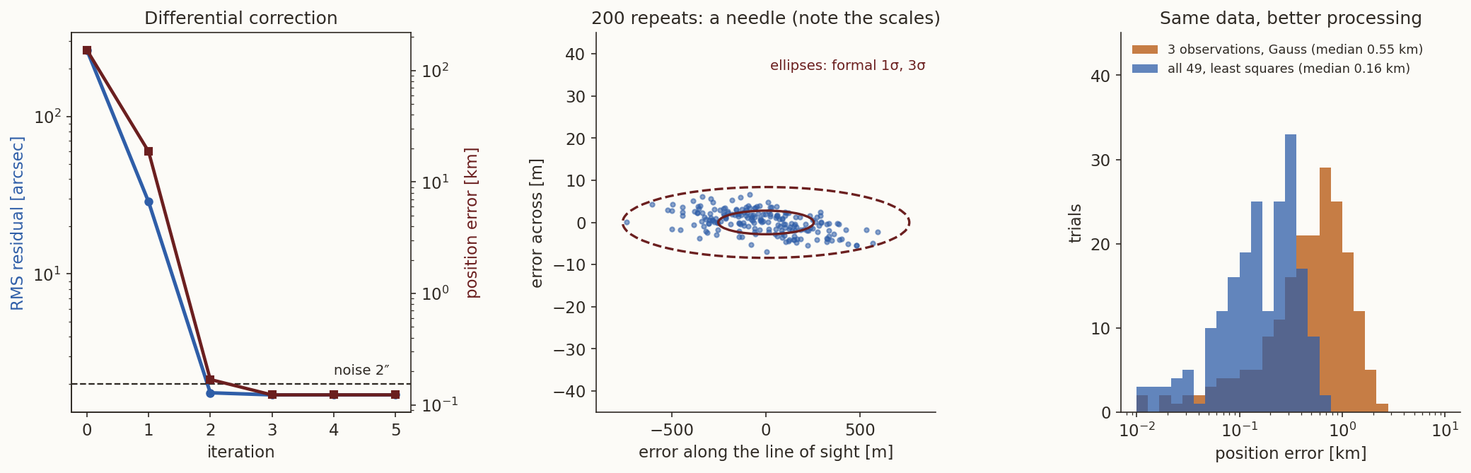
It converges in three iterations, to a residual of \(1.7''\) against the noise of \(2''\): the data fit to the noise level, neither better (which would mean over-fitting) nor worse (a wrong model). The expected value of the RMS residual for \(98\) residuals and \(6\) fitted parameters is \(2''\sqrt{92/98}=1.94''\).
The covariance Equation 24, expressed in a frame with one axis along the line of sight at \(t=0\), has the standard deviations
\[ \sigma_{\parallel}=253\ \text{m (along the line of sight)},\qquad\sigma_{\perp}=2.8\ \text{m and }2.9\ \text{m (across)}. \]
The state is determined a hundred times better across the line of sight than along it: the angles fix where the satellite is on the sky to \(3\) m, and the range remains uncertain by \(250\) m. It is the same lesson as in Section 8, now in matrix form. The actual error of this run, in the same frame, is \(123\) m along and \(-1.9\), \(1.0\) m across: consistent with the covariance.
To check that the covariance can be believed, we repeat the whole experiment \(200\) times with fresh noise (Figure 7). The scatter of the errors along and across the line of sight is \(247\) m and \(2.7\) m, \(3.0\) m, against the formal \(253\) m, \(2.8\) m, \(2.9\) m: the formal covariance predicts the actual scatter. As for the benefit of using all the data, with the same noise, Gauss’s method on the first, middle and last observation of the pass has a median position error of \(0.55\) km and \(3.0\) m/s, against \(0.16\) km and \(0.85\) m/s for the least squares on all \(49\): three times better. It does not make the range as good as the cross-range, because the arc does not contain the information: to improve on that one needs a longer arc, or another station, or a second pass.
Why is it not a contradiction that least squares finds the state to \(3\) m across the line of sight with \(2''\) of angle noise, which is \(13\) m at this range?
Answer
Each angle has a \(13\) m error, but there are \(98\) of them, and averaging \(N\) independent errors reduces the result by \(\sqrt N\). The ratio \(13.3/2.8\) says that the data are worth about \((13.3/2.8)^2\approx22\) independent measurements of the position across the line of sight (fewer than \(98\), because the same six numbers have to explain all of them). Along the line of sight there is no such averaging: the range is not in the angles, only in their curvature.What this section left out. Perturbations (the oblate Earth, drag, the Sun and Moon) are absent from the model above, and for a real pass the propagation would be numerical, with the same differential correction on top. Observations of different kinds (ranges, Doppler, angles) are combined with weights, \(\mathsf W=\mathsf R^{-1}\) in place of \(1/\sigma^2\) in Equation 23. Bad measurements are rejected by their residuals. New observations are often added one at a time, by a sequential filter, instead of in a batch; the Kalman filter (Kalman 1960) is the standard form. And a second pass, hours later, is far more informative than more observations of the first, because the along-track uncertainty grows in time while the cross-track one does not. All of this is beyond the preliminary methods, and a course of its own.
Summary
In one paragraph. An orbit needs six numbers, and the preliminary methods turn the smallest sufficient set of observations into the state. A radar with Doppler gives it directly. Three positions give it by Gibbs, with no use of the times, from the conic equation \(r+\mathbf e\cdot\mathbf r=p\), which is linear in \(\mathbf e\) and \(p\) (Equation 8); when they are close, the cancellation in Gibbs’s \(\mathbf D\) is bad, and Herrick–Gibbs uses a Taylor series in time with the gravitational acceleration at the three points (Equation 10). Two positions and the time give it by Lambert, with the time as additional information. Three directions give it by Laplace (the derivatives of the line of sight and the equation of motion at one instant) or Gauss (the Lagrange coefficients, and iterating them): both reduce to a polynomial of degree eight for \(r_2\) with a single positive root for satellites seen from the ground; Gauss, iterated, is exact for exact data. The range is carried by the curvature of the line-of-sight track, so the error of the range falls as the square of the arc, and the geometry matters (a pass through the zenith is the worst one). Least squares uses all the observations, converges from the preliminary state, and its covariance says how well each direction is determined.
| Method | Data | Uses the times? | Best when | Worst when |
|---|---|---|---|---|
| radar conversion (topocentric) | \(\rho,A,\varepsilon\) and rates, one epoch | no | a radar with Doppler is available | the rates are noisy |
| Gibbs | three positions | no | the points are far apart | they are close (cancellation) |
| Herrick–Gibbs | three positions | yes | the points are within a few tens of degrees | far apart (\(\tau^4\) error) |
| Lambert | two positions and the time | yes | two fixes and a clock | the clock is poor |
| Laplace | three directions | yes | the arc is short and the data are very accurate | long arcs (interpolation error \(\propto h^2\)) |
| Gauss | three directions | yes | the arc is moderate; with iteration, any arc | the station is nearly in the orbital plane (\(D_0\to0\)) |
| least squares | all of the above | yes | a first guess and many observations | a poor first guess |
What we left out. (i) Perturbations in the preliminary stage: the two-body model is adequate for arcs of a few minutes and wrong beyond (the \(J_2\) displacement is about \(210\) m over \(\pm240\) s). (ii) Aberration, light time, refraction, which move the observed direction by seconds of arc and are corrected before the data enter (see the topocentric note). (iii) Other angles-only methods: iterating directly on the ranges (the “double-\(r\)” idea), and methods that handle several passes and orbits with more than one revolution. (iv) Sequential filtering and the statistics of observation errors. (v) Ill-posedness: the case of a station in the orbital plane, which the formulas of this note cannot handle.
Further reading. H. D. Curtis, Orbital Mechanics for Engineering Students (Curtis 2014), the chapter on preliminary orbit determination (Gibbs’s, Lambert’s and Gauss’s methods, and the topocentric frame); D. A. Vallado, Fundamentals of Astrodynamics and Applications (Vallado 2013), the chapter on initial orbit determination (including Herrick–Gibbs, Laplace and Gauss, and their numerical behaviour); R. R. Bate, D. D. Mueller and J. E. White, Fundamentals of Astrodynamics (Bate, Mueller, and White 1971), the chapter on orbit determination from observations; P. R. Escobal, Methods of Orbit Determination (Escobal 1965), for the full treatment; and the original sources: Gauss (Gauss 1809), Laplace (Laplace 1784), Gibbs (Gibbs 1889).
The numbers of this note are checked by orbit-determination-verify.py, using the helper modules _od.py (the methods and the scenario, built on _topo.py and _uv.py) and _odmc.py (the Monte Carlo experiments, with fixed seeds); fig-od.py draws the figures.
Exercises
- Counting. How many scalar observations are needed to determine a Kepler orbit from (a) range, azimuth and elevation with their rates, (b) range, azimuth and elevation without rates, (c) azimuth and elevation only, (d) range only? (Answer: (a) six numbers at one epoch; (b) three per epoch, two epochs plus the time between them (Lambert), or three epochs; (c) two per epoch, three epochs; (d) one per epoch, six epochs, and the problem is badly conditioned.)
- Gibbs on a circle. Three positions on a circular orbit of radius \(r\), spaced by an angle \(\psi\). Show that \(\mathbf S=\mathbf 0\), \(\mathbf N=r\,\mathbf D\), \(D=r^2(2\sin\psi-\sin2\psi)\), hence \(p=r\), \(\mathbf e=\mathbf 0\), and \(v_2=\sqrt{\mu/r}\). (Hint: the three radii are equal, so \(\mathbf S=\mathbf 0\) and \(\mathbf N=r\mathbf D\); Equation 8 then gives \(\mathbf v_2=\sqrt{\mu/(rD^2)}\ \mathbf D\times\mathbf r_2/r\), and \(\lVert\mathbf D\times\mathbf r_2\rVert=D\,r\).)
- The dependence identity. Prove Equation 2 in components for three vectors in the \(xy\)-plane, \(\mathbf r_i=(x_i,y_i,0)\), with \([ij]=x_iy_j-x_jy_i\).
- Herrick–Gibbs. Show that the combination Equation 10 gives the exact velocity at \(t_2\) for the polynomial history \(\mathbf r(t)=\mathbf c_0+\mathbf c_1t+\mathbf c_2t^2+\mathbf c_3t^3+\mathbf c_4t^4\), with \(\mathbf a=\ddot{\mathbf r}\) in place of \(-\mu\mathbf r/r^3\). (Hint: the combination is linear in \(\mathbf r\) and \(\mathbf a\); check it on each power of \(t\). The \(t^3\) and \(t^4\) terms are the ones that need the acceleration.)
- The clock. Two position fixes \(600\) s apart on an orbit with \(v=7.3\) km/s. A timing error of \(1\) ms in one of them is equivalent to what position error along the track? (Answer: \(7.3\) m.)
- Unique root. Show that if \(B>0\) and \(\rho>0\) on the geometric branch, the curves Equation 13 and Equation 14 cross at most once. (Hint: differentiate both with respect to \(r\).) What does \(B<0\) do? (Answer: both derivatives are then positive, and the curves can cross several times.)
- The size of the signal. A \(2''\) error at a range of \(2410\) km is how many metres across the line of sight? (Answer: \(23.4\) m.) How many times larger than the \(2''\) noise is the out-of-plane signal \(21''\) of the first row of the table of Section 8? (Answer: \(10.6\) times; the range error of \(77\) km is the corresponding few-percent error in the curvature, magnified.)
- A zenith pass. In the helper module, call the truth state with a cross-track offset of \(0^\circ\) instead of \(5^\circ\) (a pass within \(8\) km of the zenith) and run the iterated Gauss method at \(\pm60\) s, first on exact lines of sight and then with \(2''\) of noise (300 trials). Compare with the scenario. (Answer: the exact lines of sight still give the exact orbit, to \(4\times10^{-9}\) km, but with \(2''\) of noise the median error is \(123\) km against about \(2\) km for the pass of the scenario (the table of Section 8), some \(60\) times worse; \(D_0\) is \(65\) times smaller.)
- Series for \(F\) and \(G\). Show that \(F_1G_3-F_3G_1=\tau-u\tau^3/6+O(u^2)\) from \(F\approx1-u\tau^2/2\), \(G\approx\tau-u\tau^3/6\). Then check, for equal spacing \(\tau_3=-\tau_1=60\) s and \(u=9.08\times10^{-7}\) s\(^{-2}\), that the exact value of \((F_1G_3-F_3G_1)/\tau\) is \(0.99782\), which the series reproduces to \(2\times10^{-6}\).
- Which method? For each case, name a method and say why: (a) a radar fixes three positions \(5\) s apart; (b) a radar fixes three positions \(5\) min apart; (c) a telescope gives directions every \(2\) s for \(2\) min; (d) a GPS receiver gives a position every minute, and one needs the velocity at one of them. (Answer: (a) Herrick–Gibbs; (b) Gibbs; (c) iterated Gauss on the first, middle and last directions, then least squares on all; (d) Herrick–Gibbs with the neighbouring fixes, or Lambert if only two are used.)