Lunar Trajectories: Phasing Loops and Low-Thrust Spirals
Waiting for the Moon in a loop, and climbing to it on a spiral: two ways to the Moon that trade time for something else
Where we are going
The flight to the Moon of the patched-conics note (Example 2a) is one burn and a coast: at the perigee of a \(300\) km parking orbit the vehicle gains \(3.106\) km/s, and about three days later it reaches the Moon’s sphere of influence. It has two demands. The burn must be made at the moment when the Moon is \(123.07^\circ\) ahead of the perigee, and the whole \(3.106\) km/s must be delivered in minutes. This note looks at what to do when one of the two demands cannot be met, and it gives a different answer for each.
- If the timing cannot be met, because the launch has happened and the Moon is somewhere else, the vehicle can wait. It waits on a highly eccentric Earth orbit, a phasing loop, flying it \(k\) times until the Moon is in the right place, and makes the trans-lunar burn at the perigee of the last loop. We shall find that this costs no extra \(\Delta v\): it costs time. It is the technique of the missions whose launchers could not make a direct injection.
- If short burns cannot be made, because the engine is an ion thruster that pushes with about two ten-thousandths of a newton per kilogram, there are no burns at all. The vehicle thrusts for months and spirals outward. The \(\Delta v\) is larger than for the impulsive flight, but the propellant is smaller, because the exhaust speed is five to ten times higher. Here the price is again time, now measured in months. This part is also an introduction to low-thrust flight in general, which the course has met so far only in a few formulas.
Background. The patched-conics note (its Example 2a is the transfer that the loops deliver) and the Earth–Moon system of the lunar-trajectories note; the phasing condition on a single orbit from the phasing note; the rocket equation; and, for the spiral, the energy of a circular orbit. The finite-burn side of loops (“why split a burn into several perigee burns”) is in the Chobotov note, and Edelbaum’s plane-change formula for spirals is derived in its low-thrust section.
Data and conventions. Distances in km, speeds in km/s, times in hours or days. \(\mu_\oplus=398\,600.4418\) km\(^3\)/s\(^2\), \(\mu_{\rm Moon}=4902.8\) km\(^3\)/s\(^2\), \(R_\oplus=6378.137\) km, \(R_{\rm Moon}=1737.4\) km. The Moon moves on a circle of radius \(r_{\rm Moon}=384\,400\) km at \(n_{\rm Moon}=\sqrt{(\mu_\oplus+\mu_{\rm Moon})/r_{\rm Moon}^3}=2.6653\times10^{-6}\) rad/s, which is \(13.194^\circ\) per day and a period of \(27.28\) d (the value of every note of the course; the sidereal month, \(27.32\) d, is the real Moon’s). Its sphere of influence has the radius \(r_{\rm SOI}=66\,183\) km. The parking orbit is \(300\) km high, \(r_0=6678.137\) km. Everything is planar, in the plane of the Moon’s orbit.
1 Why the timing matters
1.1 The Moon has to be at \(\phi_0\)
Measure polar angles from the perigee direction of the trans-lunar ellipse (the direction from the Earth to the burn point), counter-clockwise, the way both the vehicle and the Moon move. The ellipse is the Hohmann transfer to the Moon’s orbit, with \(a_{\rm H}=(r_0+r_{\rm Moon})/2=195\,539.1\) km, so the vehicle’s apogee is at \(180^\circ\) and it takes \(T_{\rm H}/2=119.52\) h to get there. During that time the Moon turns \(n_{\rm Moon}T_{\rm H}/2=65.71^\circ\), so for the Moon to meet the vehicle at the apogee it must be \(180^\circ-65.71^\circ=114.29^\circ\) ahead of the perigee at the burn. This is the textbook timing. To hit the Moon’s sphere of influence at the point that gives a \(100\) km perilune, Example 2a adjusts it to
\[ \phi_0=123.07^\circ , \tag{1}\]
and we take that value from there; the SOI is entered \(78.86\) h after the burn, and the burn is \(\Delta v_{\rm TLI}=v_{\rm TLI}-v_{c0}=10.8322-7.7258=3.1064\) km/s. The angle \(\phi_0\) is the requirement of a lunar transfer: the Moon’s angle \(\phi(t)\) from the perigee direction must equal \(\phi_0\) at the moment of the burn. In a time \(t\) it grows as
\[ \phi(t)=\phi_a+n_{\rm Moon}\,t , \tag{2}\]
where \(\phi_a\) is its value at \(t=0\). It moves \(13.19^\circ\) per day: a burn made a day too early or too late finds the Moon \(13^\circ\) out, and the perilune moves by thousands of kilometres (Section 2.4).
1.2 Two dials: where and when
A trans-lunar burn has two things to get right: where in its orbit the vehicle makes it, and when. From a circular parking orbit the first is free: the burn point goes round the orbit in \(90.5\) minutes, in which the Moon moves only \(0.83^\circ\), so the vehicle simply waits for the point that is \(\phi_0\) behind the Moon. The timing is then solved within one orbit, and no loop is needed. This is how a vehicle with a restartable upper stage and a parking orbit does it.
A loop is needed when the place is fixed and the time is free. This happens in four ways.
- The launcher injects the vehicle directly into an elliptic orbit, and the perigee point is wherever the ascent puts it. A parking orbit that does not exist cannot be waited in.
- The launch time of day is fixed by the plane: the plane that will contain the Moon’s position at arrival has to be reached by an ascent from a rotating Earth, once a day (see the lunar note). The perigee direction in that plane then follows from the ascent.
- The date of the launch is fixed by other things (lighting on the Moon, the availability of the range), and not by the Moon’s phase.
- The vehicle needs days in orbit, to be checked, commissioned or corrected, before it is committed to the Moon.
In each case the question is the same: injected where and when it was, the Moon at the angle \(\phi_a\), how long must the vehicle wait, and in what kind of orbit?
2 The phasing loop
2.1 The idea and its condition
Instead of the trans-lunar ellipse, the first burn, at the perigee, puts the vehicle on a smaller ellipse with the same perigee and a period \(T_{ph}\): the phasing ellipse. After \(k\) revolutions the vehicle is back at the perigee, where the second burn finishes the job and puts it on the trans-lunar ellipse. The two burns are at the same point and, as we shall see, in the same direction.
| symbol | meaning |
|---|---|
| \(\phi_a\), \(\phi_0\) | angle of the Moon from the perigee direction at the first burn; the angle it must have at the trans-lunar burn (Equation 1) |
| \(n_{\rm Moon}\), \(T_{\rm Moon}\) | the Moon’s mean motion and period, \(27.28\) d |
| \(W\), \(m\), \(k\) | the wait between the two burns; whole months added to it; number of loops |
| \(T_{ph}\), \(a_{ph}\), \(e_{ph}\), \(r_{a,ph}\), \(v_{ph}\) | period, semi-major axis, eccentricity, apogee radius and perigee speed of the phasing ellipse |
| \(r_0\), \(v_{c0}\) | the perigee radius, equal to the parking-orbit radius, and its circular speed |
| \(a_{\rm H}\), \(v_{\rm TLI}\) | the trans-lunar (Hohmann) ellipse of Example 2a and its perigee speed |
| \(\Delta v_1\), \(\Delta v_2\) | the first burn and the trans-lunar burn |
The vehicle spends \(W=k\,T_{ph}\) on the loops. The Moon must advance from \(\phi_a\) to \(\phi_0\) in that time, and it may advance by a whole number of months on top, so by Equation 2
\[ \boxed{\;W=\frac{\phi_0-\phi_a+2\pi m}{n_{\rm Moon}},\qquad T_{ph}=\frac{W}{k},\qquad m=0,1,\dots\;} \tag{3}\]
The angle \(\phi_0-\phi_a\) is taken between \(0\) and \(2\pi\), the shortest wait; \(m=1\) adds \(27.28\) d, which nobody does unless forced to. The period fixes the size of the ellipse by Kepler’s third law, and the perigee is \(r_0\) whatever the period, so
\[ a_{ph}=\left(\frac{\mu_\oplus T_{ph}^2}{4\pi^2}\right)^{1/3},\qquad r_{a,ph}=2a_{ph}-r_0,\qquad v_{ph}=\sqrt{\mu_\oplus\Bigl(\frac{2}{r_0}-\frac1{a_{ph}}\Bigr)} . \tag{4}\]
The loop must be longer than the parking orbit (\(r_{a,ph}>r_0\)) and it must stay clear of the Moon, wherever the Moon is. If the apogee is to stay at least \(1.5\,r_{\rm SOI}\) inside the Moon’s orbit, the largest apogee is
\[ r_{a,\max}=r_{\rm Moon}-1.5\,r_{\rm SOI}=285\,126\ \text{km}, \tag{5}\]
which is a loop period of at most \(6.42\) d. Waits longer than that are shared among more loops.
2.2 The loop costs no \(\Delta v\)
At the perigee the vehicle’s velocity is perpendicular to the radius, on the circle, on the phasing ellipse and on the trans-lunar ellipse alike. Both burns are therefore along the velocity, and each changes only the speed:
\[ \Delta v_1=v_{ph}-v_{c0},\qquad \Delta v_2=v_{\rm TLI}-v_{ph}, \qquad\Longrightarrow\qquad \boxed{\;\Delta v_1+\Delta v_2=v_{\rm TLI}-v_{c0}=3.1064\ \text{km/s}\;} \tag{6}\]
whatever \(v_{ph}\), that is whatever the period and the number of loops. The intermediate speed cancels. In the impulsive model a phasing loop is free. It splits the one burn into two, the first one large and the second small (the longer the loop, the smaller the second burn), and it pays in time and nothing else. The same argument covers any number of perigee burns, which is why a sequence of apogee-raising burns, as flown by several missions, costs the same \(\Delta v\) as the direct injection.
History: three Earth-orbit sequences. LADEE (NASA, 2013) was launched on 7 September 2013 by a Minotaur V that could not give the direct trans-lunar injection. It was put in a very elliptic Earth orbit, with an apogee of about \(50\) Earth radii (\(319\,000\) km, beyond the \(285\,000\) km cap used below, which is a conservative choice of this planar model), and flew three phasing loops (one account counts three and a half) before lunar orbit insertion on 6 October 2013; the price of the design was extra time in cislunar space (the mission design blog; mission and trajectory design). Chandrayaan-1 (ISRO, 2008): PSLV-C11 left it in a \(255\times22\,860\) km orbit on 22 October 2008; Earth-bound orbit-raising burns (the catalogue of the PDS lists five) raised the apogee to about \(380\,000\) km by the last, on 4 November (ISRO’s release), and it entered lunar orbit on 8 November. Chandrayaan-2 (2019) made five Earth-bound burns between 24 July and 6 August, the trans-lunar burn (\(1203\) s) on 14 August, and lunar orbit insertion on 20 August (ISRO). In these sequences the intermediate orbits do the work of phasing orbits: they set the energy and the timing together.
2.3 Worked example: three loops
Example 1. Three phasing loops before the trans-lunar burn.
Problem. A spacecraft is injected at the perigee of a phasing ellipse, \(300\) km above the Earth (\(r_0=6678.137\) km), at the moment when the Moon is \(\phi_a=35^\circ\) ahead of the perigee direction. It will make the trans-lunar burn of Example 2a, which needs the Moon \(\phi_0=123.07^\circ\) ahead, at the perigee of the third loop. Find (1) the waiting time and the period, (2) the phasing ellipse, (3) the two burns, (4) how close the vehicle comes to the Moon during the loops, (5) what the Moon and the Earth’s oblateness do to the loops.
Data. \(r_0\), \(\mu_\oplus\), \(n_{\rm Moon}\), \(r_{\rm SOI}\) as above; \(v_{c0}=7.7258\) km/s; the trans-lunar ellipse of Example 2a, \(a_{\rm H}=195\,539.1\) km, with \(v_{\rm TLI}=10.8322\) km/s at perigee; \(\phi_0=123.07^\circ\); \(k=3\).
Plan. Equation 3 gives the wait and so the period; Equation 4 the ellipse; Equation 6 the burns (and a check); then a numerical integration of the vehicle with the Earth and the Moon both pulling answers (4) and (5).
Step 1: the wait. The Moon must advance by \(\phi_0-\phi_a=123.07^\circ-35^\circ=88.07^\circ\), at \(13.1943^\circ\) per day:
\[ W=\frac{88.07^\circ}{13.1943^\circ/\text{d}}=6.675\ \text{d}=160.19\ \text{h},\qquad T_{ph}=\frac{W}{3}=2.2249\ \text{d}=53.40\ \text{h}. \]
Step 2: the phasing ellipse. From Equation 4,
\[ \begin{aligned} a_{ph}&=\left(\frac{398\,600.4\times(2.2249\times86\,400)^2}{4\pi^2}\right)^{1/3}=71\,990.9\ \text{km},\\ r_{a,ph}&=2(71\,990.9)-6678.1=137\,304\ \text{km}, \end{aligned} \]
an eccentricity \(e_{ph}=(r_{a,ph}-r_0)/(r_{a,ph}+r_0)=0.90724\) and a perigee speed \(v_{ph}=\sqrt{398\,600.4\,(2/6678.137-1/71\,990.9)}=10.6695\) km/s. The apogee, \(137\,000\) km, is well below the cap of Equation 5.
Step 3: the burns.
\[ \Delta v_1=10.6695-7.7258=2.9437\ \text{km/s},\qquad \Delta v_2=10.8322-10.6695=0.1627\ \text{km/s}, \]
and their sum is \(3.1064\) km/s, the direct injection of Example 2a, as Equation 6 says. After the second burn the vehicle is on the ellipse of Example 2a at the moment the Moon is at \(\phi_0\) (the Moon has turned \(3\,n_{\rm Moon}T_{ph}=88.07^\circ\), so \(\phi=123.07^\circ\)), and it reaches the sphere of influence \(78.86\) h later.
Step 4: the Moon during the loops. The loops are the same size in every revolution; the apogee, \(137\,300\) km on the side opposite to the perigee, is the point nearest the Moon’s orbit, and the Moon is at \(35^\circ\) to \(123^\circ\) while the apogee is at \(180^\circ\). Integrating the planar motion with the Earth and the Moon, the smallest distance to the Moon’s centre during the three loops is \(351\,724\) km, \(5.3\) sphere-of-influence radii. For the longest loop of the table below, \(k=1\) with an apogee of \(292\,816\) km, it is still \(376\,357\) km.
Step 5: what the idealisation leaves out. In the same integration the Moon’s pull raises the perigee: it returns at \(6719.6\), \(6749.1\) and \(6729.6\) km at the three passes (\(41\), \(71\) and \(51\) km up, against \(6678.137\) km with the Earth alone), each return is late by \(78\), \(76\) and \(40\) s, and the perigee direction, in the planar model, moves by \(0.008^\circ\), \(-0.011^\circ\) and \(-0.040^\circ\) at the three returns. The Earth’s oblateness (see the gravity note) acts on the line of apsides and on the plane. For \(p_{ph}=12\,737\) km and \(i=28.5^\circ\) the apse turns at \(\dot\omega=\tfrac34 n_{ph}J_2(R_\oplus/p_{ph})^2(5\cos^2 i-1)=+0.0943^\circ\) per day, and the node regresses at \(\dot\Omega=-\tfrac32 n_{ph}J_2(R_\oplus/p_{ph})^2\cos i=-0.0579^\circ\) per day: over the wait, \(+0.63^\circ\) and \(-0.39^\circ\). The two combine in the direction of the perigee, which is the burn point, and it turns in space by \(0.29^\circ\) to \(0.34^\circ\), depending on where in the plane it lies. The Moon must make up the difference, so the wait is longer by \(0.53\) to \(0.62\) h (\(0.33\%\) to \(0.39\%\)), and the condition of Equation 3 has to be corrected by that. The plane itself tilts: the orbit normal turns by \(0.18^\circ\) (about \(|\sin i\,\Delta\Omega|\)), which is \(1240\) km out of the plane of the design at the Moon’s distance. The period correction is cheap: a prograde burn of \(0.54\) m/s at the perigee lengthens the loop by \(10\) minutes (the perigee is the cheap place to change a period, as in the phasing note); the out-of-plane correction is not, and is one of the reasons for keeping the loops few and short.
The loop count is a free choice. The table gives the answer for the same wait, \(W=6.675\) d, with other values of \(k\).
| \(k\) | \(T_{ph}\) [d] | \(r_{a,ph}\) [km] | \(\Delta v_1\) [km/s] | \(\Delta v_2\) [km/s] | sum [km/s] |
|---|---|---|---|---|---|
| \(1\) | \(6.675\) | \(292\,816\) | \(3.0776\) | \(0.0288\) | \(3.1064\) |
| \(2\) | \(3.337\) | \(181\,991\) | \(3.0050\) | \(0.1014\) | \(3.1064\) |
| \(3\) | \(2.225\) | \(137\,304\) | \(2.9437\) | \(0.1627\) | \(3.1064\) |
| \(4\) | \(1.669\) | \(112\,176\) | \(2.8887\) | \(0.2177\) | \(3.1064\) |
| \(5\) | \(1.335\) | \(95\,747\) | \(2.8379\) | \(0.2685\) | \(3.1064\) |
More loops make smaller ellipses, safer from the Moon and from its perturbation, and each passes through the radiation belts and the atmosphere’s reach at the perigee once more; \(k=1\) is nearly at the Moon’s orbit. The designer’s choice is the middle.
The Moon is \(60^\circ\) behind the perigee direction at the first burn (\(\phi_a=-60^\circ\)). How long is the shortest wait, and which values of \(k\) keep the apogee below the cap of Equation 5?
What you should find
\(\phi_0-\phi_a=183.07^\circ\), so \(W=183.07^\circ/13.1943^\circ\text{/d}=13.875\) d. One loop would be \(13.9\) d long, with an apogee of \(481\,000\) km, beyond the Moon’s orbit; \(k=2\) (\(T_{ph}=6.94\) d) has \(r_{a,ph}=300\,600\) km, above the cap; \(k=3\) (\(T_{ph}=4.625\) d) has \(227\,800\) km and \(k=4\) (\(3.47\) d) has \(186\,900\) km. \(k=3\) is the least number of loops that fits.2.4 What the loops buy: every day is a launch day
Figure 1 shows the example to scale, and the clock on which it works: the Moon’s angle \(\phi(t)\) is a straight line in time, the vehicle comes back to the perigee at \(0\), \(T_{ph}\), \(2T_{ph}\) and \(3T_{ph}\), and the trans-lunar burn is made at the one of those times at which the line is at \(\phi_0\).
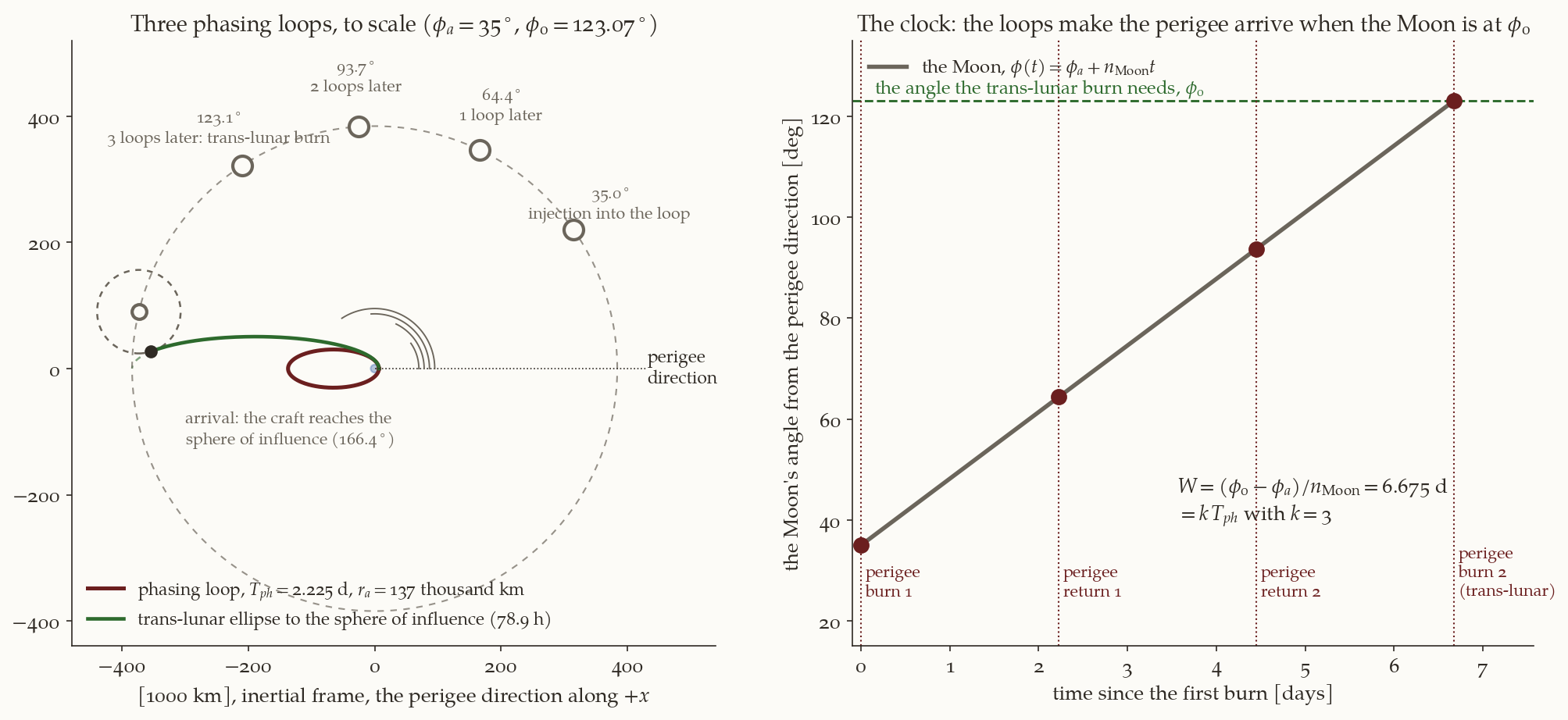
How much launch-time freedom does this give? Without a loop, and with the burn point fixed, the burn has to be made when \(\phi=\phi_0\) to within a fraction of a degree. With the patched-conic solution of Example 2a, the perilune altitude is \(100\) km at \(\phi_0\), \(1094\) km one degree later and an impact (\(-634\) km) one degree earlier: \(730\) to \(990\) km per degree of \(\phi_0\), and a correction of that much is expensive. One degree of the Moon’s motion is \(1.82\) h, so the Moon spends an hour or two in the usable range, once a month. With \(k\) loops of at most \(6.42\) d (Equation 5), any wait up to \(6.42\,k\) days can be filled. Figure 2 shows that \(k=4\) covers waits up to \(25.7\) d and \(k=5\) covers \(32.1\) d, longer than a month: five loops can serve any phase of the Moon. The only cost of a longer wait is more orbits to fly (and, in a real mission, more time for things to go wrong).
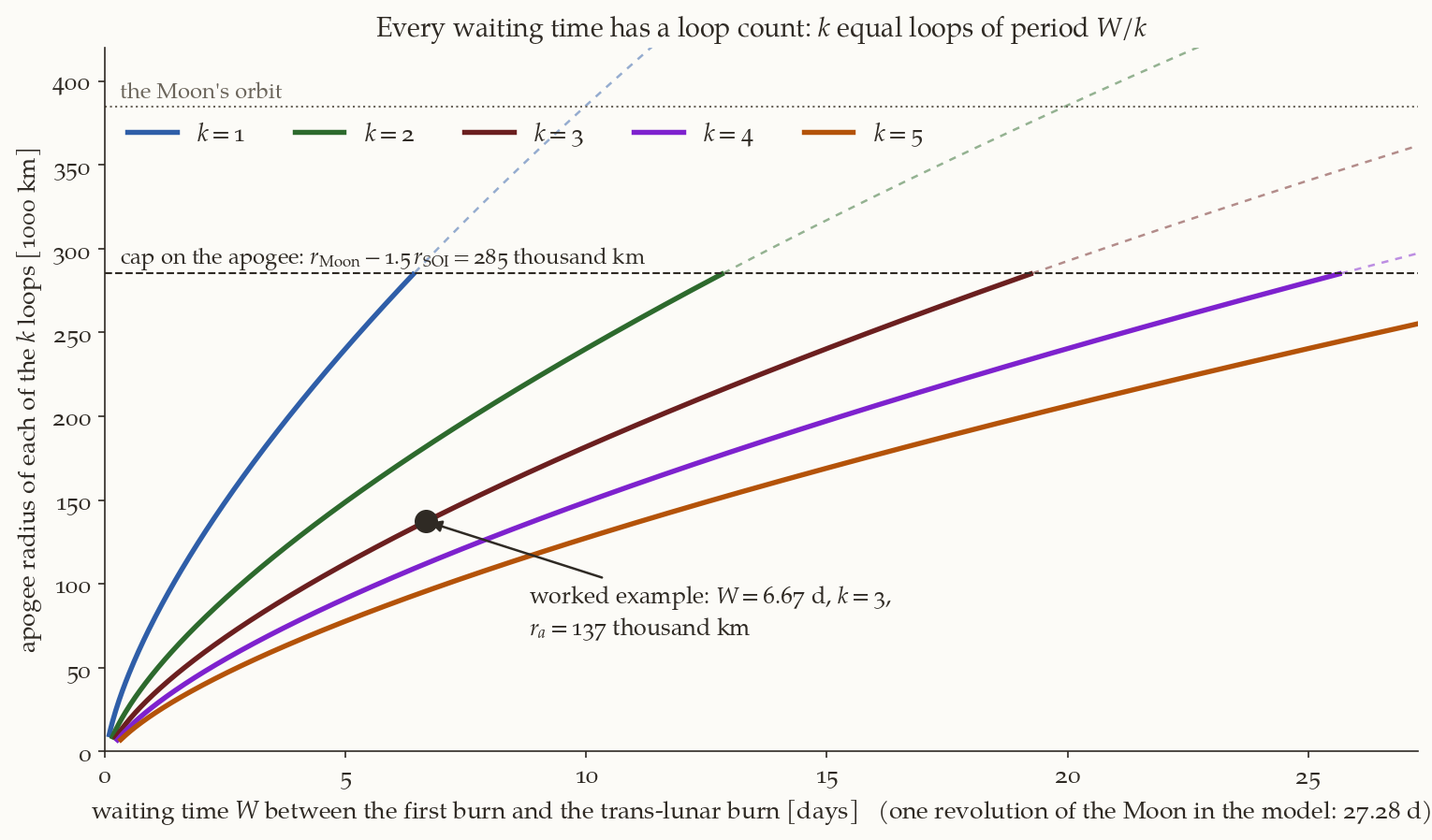
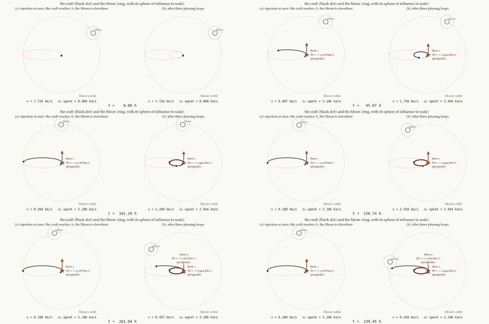
Figure 3 shows the difference in motion. Both panels start at the same instant, with the Moon \(35^\circ\) ahead. On the left the whole injection is made at once: the vehicle reaches the apogee A at \(119.5\) h, and the Moon, which is \(65.7^\circ\) further on, is \(79.3^\circ\) short of it. On the right the vehicle flies three loops, and the second burn is small.
2.5 What it costs in a real mission
The impulsive model said “nothing”. Four things say otherwise.
Finite burns. A real engine takes minutes, and a burn that is long compared with the time near the perigee loses \(\Delta v\) to gravity (the Chobotov note works this out). The cure is the same technique: split the burn into several made at successive perigees, which is what a phasing loop does. In the experiment of that note (the table in its section on several perigee burns), an engine of thrust-to-weight \(T/W_0=0.03\) that raises a \(278\) km orbit to a geosynchronous apogee loses \(499.8\) m/s in one burn (\(1.9\) h) and \(21.8\) m/s in eight (\(23.8\) h). So for a stage of modest thrust-to-weight ratio the loops save \(\Delta v\) against one long burn, and that is a main reason why Earth-orbit sequences are flown at all: the real exchange is time for \(\Delta v\), the opposite of the impulsive model’s “time for nothing”.
Perturbations. The Moon’s pull changed the perigee by tens of kilometres in three loops (Step 5), the Earth’s oblateness turns the line of apsides and tilts the plane (\(0.18^\circ\), \(1240\) km at the Moon, in the example), and the Sun does as much as the Moon at these apogees. The perigee is raised or lowered, and a lowered perigee can bring the vehicle into the atmosphere. The loops need tracking and small corrections, in the plane and out of it.
Exposure. Each perigee passage crosses the radiation belts, and a loop of \(2.2\) d has two crossings per period.
Moon’s neighbourhood. The cap of Equation 5 keeps the apogee away from the Moon; a \(k=1\) loop of \(6.7\) d reaches \(293\,000\) km and the geometry is no longer simple.
The answer to the first question of the note is therefore: the wait is Equation 3, the loops are the shortest that keep the apogee under the cap, and the cost in \(\Delta v\) is zero on paper and, if anything, negative in practice.
3 Low thrust: an introduction
3.1 What “low thrust” means
What matters about an engine is not its thrust \(F\) but the acceleration \(a_T=F/m\) it gives, compared with gravity’s, \(g=\mu_\oplus/r^2\). Their ratio is
\[ \kappa=\frac{a_T}{g}=\frac{a_T\,r^2}{\mu_\oplus}. \tag{7}\]
(The letter \(\varepsilon\) stays for the specific energy, as everywhere else in the course; \(\kappa\) is used for this ratio only.)
A chemical stage has \(\kappa\) between \(0.03\) and \(10\) at the start of a burn: it burns for minutes, and the burn is nearly an impulse when \(\kappa\gtrsim0.5\). For \(\kappa\) from \(0.01\) to \(0.1\) the burn is long enough to lose a lot to gravity, and one splits it into several, as the loops above do. An ion or Hall thruster has \(\kappa\approx10^{-5}\) to \(10^{-3}\): it can only be on for months, at an acceleration that moves the vehicle by a negligible amount in one orbit, and the orbit changes slowly and continuously.
The reason for building such engines is the exhaust speed, \(c=g_0I_{sp}\), \(g_0=9.80665\times10^{-3}\) km/s\(^2\). A chemical stage has \(I_{sp}\approx300\) s, \(c\approx3\) km/s; an electric thruster has \(1500\) to \(3000\) s, \(c\approx15\) to \(30\) km/s, and by the rocket equation the propellant for a given \(\Delta v\) is
\[ \frac{m_p}{m_0}=1-e^{-\Delta v/c} \tag{8}\]
so \(10\) times the exhaust speed needs far less than a tenth of the propellant when the \(\Delta v\) is of order \(c\). The price is that the thrust is small, for reasons of power (Section 3.5), and the transfer takes a long time.
History: SMART-1. ESA’s SMART-1 was launched in September 2003 and used a Snecma PPS-1350-G Hall thruster, of \(68\) mN and a specific impulse of \(1640\) s, to spiral up from its transfer orbit, the engine on for roughly a third to a half of every orbit. It was captured by the Moon on 15 November 2004. ESA’s status report of 26 October 2004 gives the account at that date: \(58.8\) kg of xenon had been used, the thruster had been on for \(3648\) h, and the speed gained was \(2737\) m/s (status report; ESA). From those figures alone, the average thrust acceleration was \(2.737/(3648\times3600)=2.08\times10^{-7}\) km/s\(^2\), which is the value we use below. It did not start in a circular orbit and it did not end in one: the mission timeline lists a “final lunar resonance and capture”, so the Earth-only spiral of this note is a model of the first part of its climb.
3.2 The spiral and its speed
Suppose a vehicle on a circular orbit of radius \(r\) thrusts along its velocity with the acceleration \(a_T\), small enough that the orbit stays almost circular (this will be shown in Section 3.3). The energy of the orbit is \(\varepsilon=-\mu_\oplus/(2r)\), and it changes at the rate at which the thrust does work,
\[ \frac{d\varepsilon}{dt}=\mathbf a_d\cdot\mathbf v=a_Tv . \tag{9}\]
On a circular orbit \(v^2=\mu_\oplus/r\), so \(\varepsilon=-v^2/2\) and \(d\varepsilon/dt=-v\,\dot v\). Setting this equal to \(a_Tv\),
\[ \boxed{\;\frac{dv_c}{dt}=-a_T\;} \tag{10}\]
Thrusting forward makes the circular speed fall at exactly the rate of the thrust acceleration. The paradox is only apparent: the thrust does positive work, so the total energy rises, but in a circular orbit the kinetic energy is \(-\varepsilon\), so a rise of the total energy by \(\delta\varepsilon\) means a fall of the kinetic energy by \(\delta\varepsilon\) and a rise of the potential energy by twice that. The vehicle slows down because it climbs.
The consequences are immediate. The speed falls linearly in time and the radius follows from the circular-speed relation \(r=\mu_\oplus/v_c^2\):
\[ v_c(t)=v_{c1}-a_Tt,\qquad r(t)=\frac{\mu_\oplus}{(v_{c1}-a_Tt)^2} . \tag{11}\]
A spiral from a circle of radius \(r_1\) to a circle of radius \(r_2>r_1\) therefore costs
\[ \boxed{\;\Delta v=v_{c1}-v_{c2}\;},\qquad t=\frac{\Delta v}{a_T}\quad\text{(constant }a_T\text{)} . \tag{12}\]
A spiral between coplanar circles costs the difference of the circular speeds, not the sum of two impulses. For the number of revolutions, each takes \(2\pi r/v_c\), so the revolution rate is \(v_c/(2\pi r)=v_c^3/(2\pi\mu_\oplus)\) (using \(r=\mu_\oplus/v_c^2\)), and with \(dt=-dv_c/a_T\)
\[ N=\int_0^t\frac{v_c^3}{2\pi\mu_\oplus}\,dt=\frac{1}{2\pi\mu_\oplus a_T}\int_{v_{c2}}^{v_{c1}}v_c^3\,dv_c=\frac{v_{c1}^4-v_{c2}^4}{8\pi\mu_\oplus a_T}=\frac{1}{8\pi\kappa_1}\Bigl[1-\Bigl(\frac{r_1}{r_2}\Bigr)^2\Bigr] , \tag{13}\]
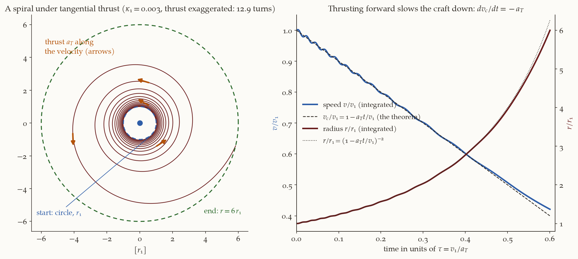
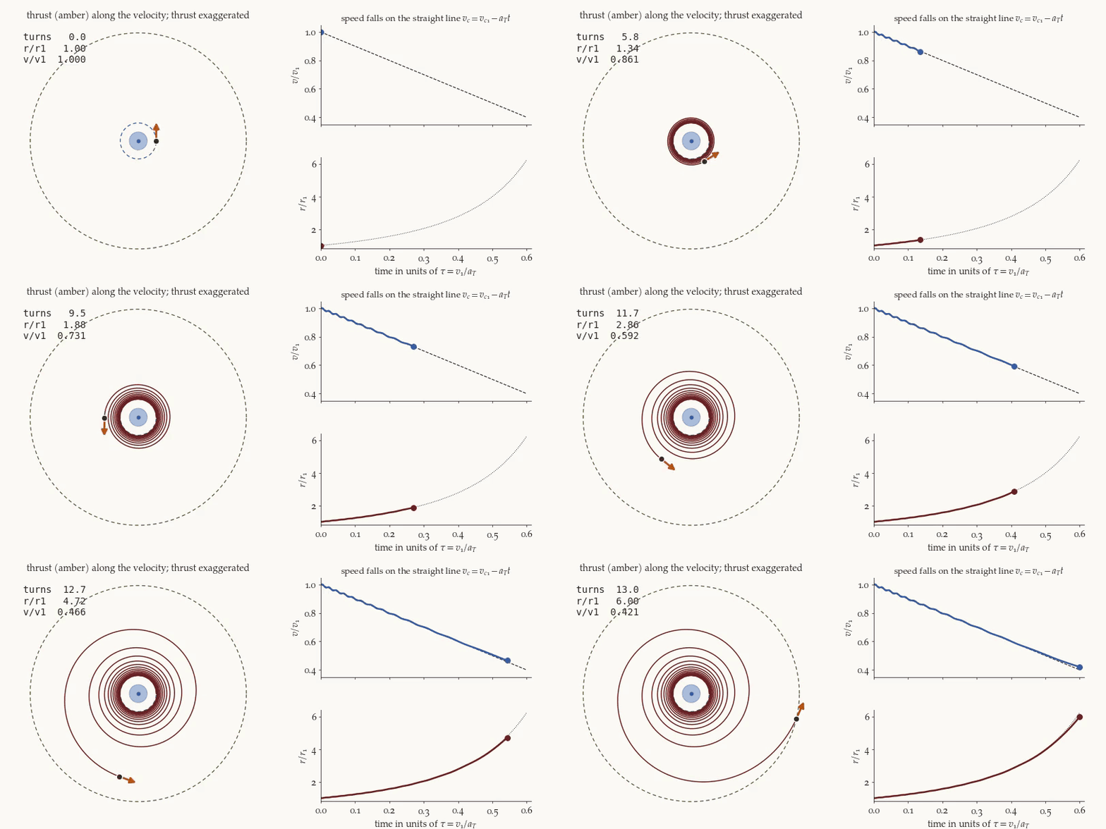
with \(\kappa_1=a_Tr_1^2/\mu_\oplus\) from Equation 7. The shape of the spiral depends on \(\kappa_1\) alone: Figure 4 draws one with \(\kappa_1=0.003\) (about \(130\) times SMART-1’s), where \(12.9\) turns take the radius from \(r_1\) to \(6r_1\), and shows the speed on its straight line.
Against the Hohmann transfer. The same two circles, joined impulsively by a Hohmann transfer, cost \(\Delta v_H=\Delta v_1+\Delta v_2\), and for LEO to the Moon’s orbit that is \(3.9365\) km/s against the spiral’s \(v_{c1}-v_{c2}=7.7258-1.0183=6.7075\) km/s: \(70\%\) more.
The reason is the speed at which the energy is bought. Every unit of \(\Delta v\) delivered at the speed \(v\) raises the energy by \(v\) per unit mass, \(d\varepsilon=v\,d(\Delta v)\) (Equation 9), so the \(\Delta v\) for a given energy gain is \(\int d\varepsilon/v\), and the higher the speed at the burn the cheaper it is: the Oberth effect of the impulsive-model note. From LEO to a circle at \(100\,000\) km the energy gain is \(\tfrac12\mu_\oplus(1/r_1-1/r_2)=27.85\) km\(^2\)/s\(^2\) for either route. An impulse along the velocity buys its energy at the mean of the speeds before and after it, \(\Delta\varepsilon=v\,\Delta v+\tfrac12\Delta v^2\): the first Hohmann burn, from \(7.73\) to \(10.58\) km/s, at \(9.15\) km/s, and the second, from \(0.71\) to \(2.00\) km/s, at \(1.35\) km/s. Together they buy the \(27.85\) km\(^2\)/s\(^2\) for \(4.1427\) km/s, which is \(6.72\) km/s of energy for each km/s of \(\Delta v\). The spiral can only push at the circular speed of the orbit it is on, falling from \(7.73\) to \(2.00\) km/s, an average of \(4.86\) km/s (\(27.85/5.7293\)), and the same energy then costs \(5.7293\) km/s. The spiral pays for having no good place to burn.
3.3 How circular does the spiral stay?
The derivation assumed a circular orbit throughout. The orbit is perturbed from a circle at every instant, and we have to show by how much. The eccentricity vector is \(\mathbf e=(\mathbf v\times\mathbf h)/\mu_\oplus-\hat{\mathbf r}\), with \(\mathbf h=\mathbf r\times\mathbf v\), and with an extra acceleration \(\mathbf a_d\) the equations of motion are \(\dot{\mathbf r}=\mathbf v\), \(\dot{\mathbf v}=-\mu_\oplus\mathbf r/r^3+\mathbf a_d\), so \(\dot{\mathbf h}=\mathbf r\times\mathbf a_d\). Differentiating, the two-body terms cancel (this is why \(\mathbf e\) is constant without \(\mathbf a_d\)) and what is left is
\[ \dot{\mathbf e}=\frac{1}{\mu_\oplus}\Bigl[\mathbf a_d\times\mathbf h+\mathbf v\times(\mathbf r\times\mathbf a_d)\Bigr] =\frac{1}{\mu_\oplus}\Bigl[2(\mathbf v\cdot\mathbf a_d)\,\mathbf r-(\mathbf r\cdot\mathbf a_d)\,\mathbf v-(\mathbf r\cdot\mathbf v)\,\mathbf a_d\Bigr], \tag{14}\]
by the identity \(\mathbf A\times(\mathbf B\times\mathbf C)=\mathbf B(\mathbf A\cdot\mathbf C)-\mathbf C(\mathbf A\cdot\mathbf B)\) applied to both terms. For a tangential acceleration, \(\mathbf a_d=a_T\hat{\mathbf v}\), on a circle (\(\mathbf r\cdot\mathbf v=0\), \(\mathbf r\cdot\mathbf a_d=0\), \(\mathbf v\cdot\mathbf a_d=va_T\), \(rv^2=\mu_\oplus\)):
\[ \dot{\mathbf e}=\frac{2va_T\,r}{\mu_\oplus}\,\hat{\mathbf r}=\frac{2a_T}{v}\,\hat{\mathbf r}. \tag{15}\]
(Its component along the periapsis direction, \(2a_T\cos f/v\), is the circular limit of the scalar equation \(\dot e=(2/v)(e+\cos f)a_T\) of the Gauss equations in tangential–normal form.) The vector \(\hat{\mathbf r}=(\cos\theta,\sin\theta)\) turns with the vehicle, \(\theta\) being its polar angle, at the mean motion \(n=v/r\), so \(\dot{\mathbf e}\,dt=(2a_T/vn)\,\hat{\mathbf r}\,d\theta\) with \(d\theta=n\,dt\), and \(2a_T/(vn)=2a_Tr^2/\mu_\oplus=2\kappa\), the ratio of Equation 7. Over a short stretch of the spiral \(\kappa\) is constant, and integrating from \(\mathbf e=0\) at \(\theta=0\),
\[ \mathbf e=2\kappa\,(\sin\theta,\ 1-\cos\theta),\qquad |\mathbf e|=4\kappa\,\Bigl|\sin\frac{\theta}{2}\Bigr| . \tag{16}\]
For constant \(\kappa\) the eccentricity vector goes round a circle of radius \(2\kappa\) that touches the origin, oscillating between \(0\) and \(4\kappa\) in every revolution. But along the spiral \(\kappa\) grows as \(r^2\), and the circle does not simply grow with it. Write \(\hat{\mathbf r}=d\hat{\mathbf s}/d\theta\) with \(\hat{\mathbf s}=(\sin\theta,-\cos\theta)\) (the vector \(\hat{\mathbf r}\) turned \(90^\circ\) backwards), and integrate by parts:
\[ \mathbf e=\int_0^\theta2\kappa\,\hat{\mathbf r}\,d\theta =2\kappa(r)\,\hat{\mathbf s}+2\kappa_1\,\hat{\mathbf j}+O(\kappa^2),\qquad\hat{\mathbf j}=(0,1), \tag{17}\]
where \(\kappa_1\) is the initial value, and the integral that is left, \(-\int2\,(d\kappa/d\theta)\,\hat{\mathbf s}\,d\theta\), is of order \(\kappa^2\) because \(d\kappa/d\theta=4\kappa^2\) (the radius grows by \(4\pi\kappa\) of itself in a revolution, and \(\kappa\propto r^2\)). Two terms remain. The forced one, \(2\kappa(r)\,\hat{\mathbf s}\), has the length \(2\kappa\) at the present radius and keeps \(90^\circ\) behind the vehicle. The free one, \(2\kappa_1\hat{\mathbf j}\), is a constant: the remnant of the abrupt start, which cancels the forced term at \(\theta=0\) where \(\mathbf e=0\), and which is small, \(2\kappa_1=4.7\times10^{-5}\) in the example below. So
\[ \bigl|\,|\mathbf e|-2\kappa(r)\,\bigr|\le2\kappa_1,\qquad |\mathbf e|\le4\kappa(r), \]
the second because \(\kappa(r)\ge\kappa_1\), with equality only at the start. After the first revolutions, when \(\kappa(r)\gg\kappa_1\), \(e\approx2\kappa(r)\). (If the initial velocity is adjusted to cancel the remnant, which takes a small radial velocity, \(|\mathbf e|=2\kappa(r)\) from the start.)
What the steady eccentricity is. The forced vector points \(90^\circ\) behind the vehicle, so the periapsis of the osculating orbit is \(90^\circ\) behind it, and the vehicle is at the true anomaly \(f=90^\circ\). On an orbit of small eccentricity the radial speed there is \(v_r=(\mu_\oplus/h)\,e\sin f\approx e\,v\). With \(e=2\kappa\),
\[ v_r=2\kappa\,v=\frac{2a_Tr^2}{\mu_\oplus}\sqrt{\frac{\mu_\oplus}{r}}=\frac{2a_T\,r^{3/2}}{\sqrt{\mu_\oplus}} , \]
which is the climb rate \(\dot r\) that the energy equation gives (Exercise 4). The eccentricity \(2\kappa\) is not a distortion of the path. The path is very nearly a circle at every instant (it climbs \(4\pi\kappa r\) in a revolution); the osculating ellipse is slightly eccentric only because the velocity is not quite perpendicular to the radius. The eccentricity is the flight-path angle, \(\gamma=v_r/v=2\kappa\). The orbit is almost circular when \(\kappa\ll1\).
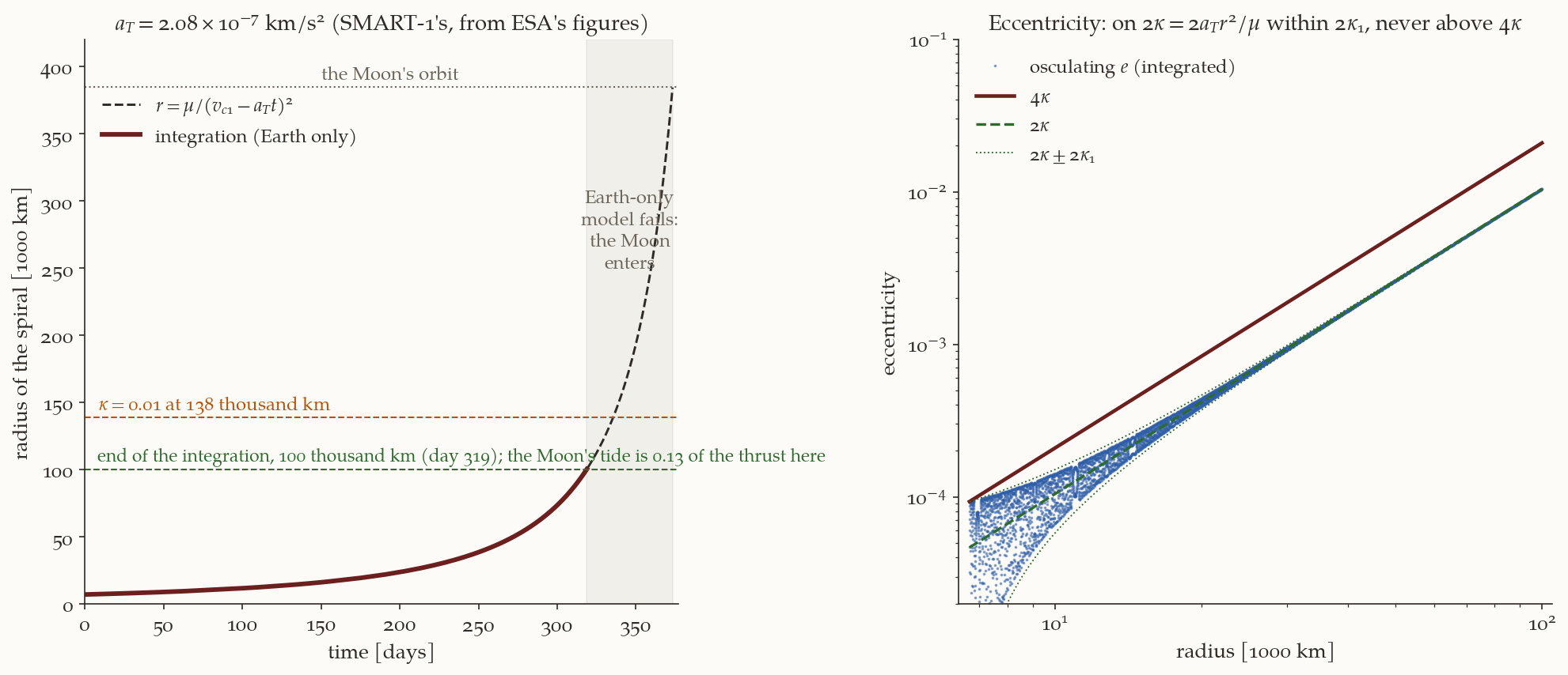
A numerical integration at a SMART-1-class acceleration, \(a_T=2.08\times10^{-7}\) km/s\(^2\) (\(\kappa_1=2.33\times10^{-5}\) at the \(300\) km orbit), from \(r_1=6678\) km to \(100\,000\) km, confirms all of it (Figure 6). The integrated time is \(318.81\) d against \(318.80\) d from Equation 12 (\(0.003\%\)), and the number of revolutions is \(1702.10\) against \(1702.09\) from Equation 13. The osculating eccentricity stays within \(2\kappa_1\) of \(2\kappa(r)\) at every sample (the ratio \(|e-2\kappa|/2\kappa_1\) reaches \(1.000\) at the start and is at most \(0.993\) after the first revolutions), never exceeds \(4\kappa(r)\) (the largest ratio is \(0.994\)), and ends at \(0.01042\) against \(2\kappa=0.01044\); the radial speed is \(2\kappa v\) to within \(2\kappa_1v\). For constant \(\kappa\) (\(\kappa_1=10^{-4}\), two revolutions) the vector itself follows Equation 16 to \(1.3\times10^{-6}\), the growth of \(\kappa\), and Equation 17 follows the vector for growing \(\kappa\) to \(2.6\times10^{-7}\).
3.4 Where the Earth-only model stops
Two things limit the spiral before the vehicle reaches the Moon, and they are different.
The orbit stops being circular. The acceleration \(a_T\) is constant and gravity falls as \(1/r^2\), so \(\kappa=a_Tr^2/\mu_\oplus\) grows as \(r^2\): for \(a_T=2.08\times10^{-7}\) km/s\(^2\) it is \(2.3\times10^{-5}\) at LEO, \(0.0052\) at \(100\,000\) km, \(0.01\) at \(138\,000\) km and \(0.077\) at the Moon’s distance. Since \(e\approx2\kappa\) is the flight-path angle of the climb, the spiral there climbs at \(2\kappa=0.154\) rad, \(8.8^\circ\) above the horizontal, and the orbit is no longer close to a circle: the model fails of its own accord, before the Moon is reached.
The Moon pulls. The Moon’s differential acceleration at the vehicle, on the Moon’s side, \(\mu_{\rm Moon}[(r_{\rm Moon}-r)^{-2}-r_{\rm Moon}^{-2}]\), is \(13\%\) of the thrust acceleration at \(100\,000\) km, \(53\%\) at \(200\,000\) km and equal to it at \(241\,800\) km (the lunar tide of the patched-conics note; see also the three-body note). Close to the Moon its direct pull equals the thrust within \(153\,500\) km, \(2.3\) sphere-of-influence radii.
So the analytic spiral is trustworthy to about \(100\,000\) km. That is \(85\%\) of the \(\Delta v\) and of the time of the whole spiral to the Moon’s distance (\(5.73\) of \(6.71\) km/s). Beyond it the vehicle is in a three-body problem and the end of the journey needs an integration (Section 3.7).
3.5 Propellant, thrust and power
Two kinds of time formula are in use, and they mean different things. With a constant thrust acceleration \(a_T\), Equation 12 gives \(t=\Delta v/a_T\). A real engine has a constant thrust \(F\), and the mass falls as the propellant is used, so the acceleration rises. For a constant exhaust speed \(c=g_0I_{sp}\) the mass flow is \(\dot m=F/c\), \(m(t)=m_0-Ft/c\), and \(\Delta v=\int F\,dt/m=c\ln(m_0/m)\) (the rocket equation, Equation 8), which gives the time
\[ t=\frac{c\,m_0}{F}\Bigl(1-e^{-\Delta v/c}\Bigr). \tag{18}\]
This is shorter than \(\Delta v/a_{T,0}\), with \(a_{T,0}=F/m_0\) the acceleration at the start, because the acceleration grows. The revolution count of Equation 13 assumed constant \(a_T\) as well; with falling mass one integrates \(v_c^3/(2\pi\mu_\oplus)\) over the time with \(v_c=v_{c1}-c\ln(m_0/m)\).
The thrust is limited by power. A thruster that turns an electrical power \(P\) into a jet of mass flow \(\dot m\) and speed \(c\) with an efficiency \(\eta\) has \(\eta P=\tfrac12\dot mc^2=\tfrac12Fc\), so
\[ F=\frac{2\eta P}{c}=\frac{2\eta P}{g_0I_{sp}}. \tag{19}\]
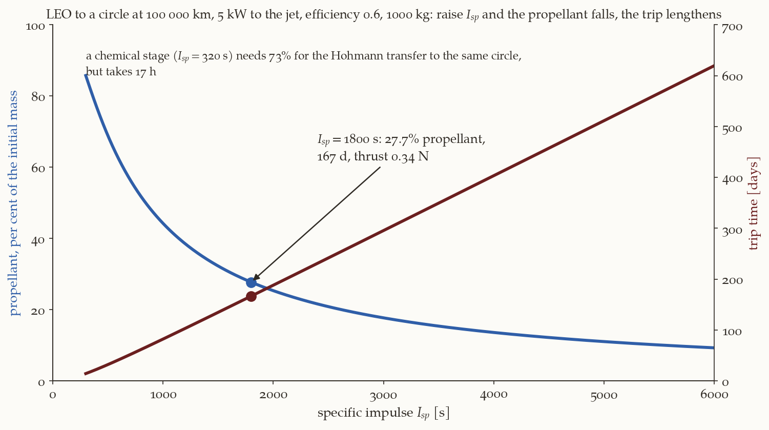
For a given power, the thrust falls as \(1/I_{sp}\): doubling the exhaust speed halves the thrust. With Equation 18 the time is \(t=c^2m_0(1-e^{-\Delta v/c})/(2\eta P)\), which rises with \(c\) (for \(c\gg\Delta v\) it is \(c\,m_0\Delta v/(2\eta P)\), proportional to \(I_{sp}\)), while the propellant falls. Figure 7 is the trade. It has no optimum, because the model has no mass for the power system. A real design includes the specific mass of the solar arrays (kg per kW), which grows with the power, and a minimum of the total mass or of the trip time appears at a finite \(I_{sp}\); the figure’s trend is still the guide.
3.6 Worked example: an electric tug
Example 2. LEO to \(100\,000\) km with \(5\) kW.
Problem. A spacecraft of wet mass \(m_0=1000\) kg in a \(300\) km circular orbit has an electric thruster with \(P=5\) kW, an efficiency \(\eta=0.6\) and \(I_{sp}=1800\) s. It spirals to a circle of radius \(100\,000\) km, where the Earth-only model stops. Find (1) the \(\Delta v\), (2) the thrust and the initial acceleration, (3) the propellant and the time, (4) the comparison with a chemical Hohmann transfer to the same circle with \(I_{sp}=320\) s.
Data. \(r_1=6678.137\) km, \(r_2=100\,000\) km, \(\mu_\oplus=398\,600.4\) km\(^3\)/s\(^2\), \(g_0=9.80665\times10^{-3}\) km/s\(^2\); \(v_{c1}=7.7258\) km/s, \(v_{c2}=\sqrt{\mu_\oplus/r_2}=1.9965\) km/s.
Plan. Equation 12 for the \(\Delta v\); Equation 19 for the thrust; Equation 8 and Equation 18 for the propellant and the time; the Hohmann transfer for the comparison.
Step 1: the \(\Delta v\). \(\Delta v=v_{c1}-v_{c2}=7.7258-1.9965=5.7293\) km/s.
Step 2: thrust and acceleration. \(c=g_0I_{sp}=9.80665\times10^{-3}\times1800=17.652\) km/s, \(F=2\eta P/c=2(0.6)(5000)/17\,652\ \text{m/s}=0.3399\) N, and \(a_{T,0}=F/m_0=3.399\times10^{-4}\) m/s\(^2=3.40\times10^{-7}\) km/s\(^2\), \(\kappa_1=3.8\times10^{-5}\).
Step 3: propellant and time. Equation 8: \(m_p/m_0=1-e^{-5.7293/17.652}=1-e^{-0.3246}=0.2772\), so \(277\) kg of propellant and \(723\) kg left. Equation 18:
\[ t=\frac{c\,m_0}{F}\bigl(1-e^{-\Delta v/c}\bigr)=\frac{17\,652\times1000}{0.3399}\times0.2772=1.439\times10^{7}\ \text{s}=166.6\ \text{d}. \]
(With the acceleration frozen at its initial value the time would be \(5.7293/3.399\times10^{-7}=195.1\) d: the rising acceleration saves \(29\) days.)
Step 4: the chemical stage. The Hohmann transfer from \(6678.137\) km to \(100\,000\) km has \(a_t=53\,339\) km, \(\Delta v_1=2.8526\) km/s, \(\Delta v_2=1.2901\) km/s, a total of \(4.1427\) km/s, in \(\pi\sqrt{a_t^3/\mu_\oplus}=17.03\) h. At \(I_{sp}=320\) s the propellant is \(1-e^{-4.1427/3.1381}=73.3\%\) of the initial mass.
| \(\Delta v\) [km/s] | \(I_{sp}\) [s] | propellant | time | |
|---|---|---|---|---|
| Hohmann, chemical | \(4.1427\) | \(320\) | \(73.3\%\) | \(17.0\) h |
| spiral, electric | \(5.7293\) | \(1800\) | \(27.7\%\) | \(166.6\) d |
What this shows. \(\Delta v\) is no longer the figure of merit: the spiral has the larger one and the smaller propellant, because the exhaust speed is \(5.6\) times higher. The saving of propellant is bought with time, and with the radiation of the belts the vehicle spirals through for months.
Take the engine of Example 2 at \(I_{sp}=3000\) s, with the same \(5\) kW and \(\eta=0.6\). What are the thrust, the propellant and the time?
What you should find
\(F=2(0.6)(5000)/29\,420=0.204\) N, \(m_p/m_0=1-e^{-5.7293/29.420}=17.7\%\), and \(t=295\) d. Against the \(1800\) s engine: \(10\) kg less propellant out of every \(100\) kg, and \(128\) days more.3.7 Reaching the Moon
An all-electric journey to the Moon has three parts: the Earth-only spiral, which we can calculate, up to about \(100\,000\) km; the part in which the Moon interferes, which needs a three-body integration and, as SMART-1 showed, lunar resonances and ballistic capture; and the spiral down around the Moon, to which the same theory applies with \(\mu_{\rm Moon}\) in place of \(\mu_\oplus\). For the last, the thrust is against the velocity, the speed rises on the way down, and the cost is \(\Delta v=v_{c,\rm low}-v_{c,\rm high}\): for a \(100\) km circular lunar orbit, \(v_c=1.6335\) km/s, from the edge of the sphere of influence (\(0.2722\) km/s) it is \(1.3613\) km/s, and from \(15\,350\) km, where \(\kappa=0.01\) for this thrust, \(1.0684\) km/s, in \(59\) days at \(2.08\times10^{-7}\) km/s\(^2\).
The table compares three ways of reaching a \(100\) km circular lunar orbit. The numbers are not like for like unless read with their labels: each row says what its \(\Delta v\) buys.
| route | what the \(\Delta v\) buys | \(\Delta v\) [km/s] | \(I_{sp}\) [s] | propellant | time |
|---|---|---|---|---|---|
| direct (Example 2a) | trans-lunar burn \(3.1064\) and capture \(0.7949\), all impulsive | \(3.9013\) | \(320\) | \(71.2\%\) | \(4.1\) d |
| phasing loops (Example 1) | the same burns, split in two at the perigee | \(3.9013\) | \(320\) | \(71.2\%\) | \(6.7+4.1\) d |
| all-electric, idealised | Earth spiral to \(r_{\rm Moon}\) (\(6.7075\)) and spiral down from the sphere of influence (\(1.3613\)) | \(8.0688\) | \(1800\) | \(36.7\%\) | \(449\) d |
The phasing loop does not change the propellant of the direct flight but changes when it flies; the electric route halves the propellant and takes over a year. The real SMART-1, which began in a transfer orbit and used the Moon’s gravity to end its climb, is reported with a total \(\Delta v\) of \(3.5\) to \(3.9\) km/s (the figures differ between sources), about that of the chemical route.
Plane change. The Moon’s orbital plane is inclined to the equator by \(18.3^\circ\) to \(28.6^\circ\), so a spiral from a LEO of a different inclination also has to turn its plane. For low-thrust spirals Edelbaum’s formula, derived in the Chobotov note, replaces Equation 12 by \(\Delta v=\sqrt{v_{c1}^2+v_{c2}^2-2v_{c1}v_{c2}\cos(\pi\Delta i/2)}\). For the spiral of Example 2, \(\Delta i=10^\circ\) makes the \(\Delta v\) \(5.829\) km/s instead of \(5.729\) (an increase of \(1.7\%\)), and \(28.5^\circ\) makes it \(6.463\) km/s (\(13\%\) more).
Summary
In one paragraph. A lunar transfer needs the Moon at the angle \(\phi_0\) from the perigee at the moment of the trans-lunar burn. When the vehicle is injected with the Moon at \(\phi_a\), it may wait in \(k\) equal phasing loops of period \(T_{ph}=(\phi_0-\phi_a)/(k\,n_{\rm Moon})\), with the same perigee, and make the trans-lunar burn at the last perigee. Both burns are tangential at that perigee, so in the impulsive model they add up to the direct injection, \(3.1064\) km/s: the loop costs time, not \(\Delta v\). Five loops under an apogee cap serve every phase of the Moon. In a real mission the loops reduce the gravity loss of a weak engine, and they expose the vehicle to perturbations and to the radiation belts at each perigee. A low-thrust spiral between circular orbits obeys \(dv_c/dt=-a_T\): the circular speed falls at the thrust acceleration, so \(\Delta v=v_{c1}-v_{c2}\), \(t=\Delta v/a_T\), and the revolutions are \((v_{c1}^4-v_{c2}^4)/(8\pi\mu_\oplus a_T)\). The osculating eccentricity settles on \(e\approx2\kappa\) (never above \(4\kappa\)), \(\kappa=a_Tr^2/\mu_\oplus\): it is the flight-path angle of the climb, \(v_r/v\), not a distortion of the path; \(\kappa\) grows as \(r^2\), and the Earth-only model holds to about \(100\,000\) km for an acceleration like SMART-1’s (\(85\%\) of the \(\Delta v\) to the Moon). The spiral costs more \(\Delta v\) than the impulsive transfer (\(38\%\) more to \(100\,000\) km) and much less propellant, because \(I_{sp}\) is about six times higher; the price is a trip of months, and for a fixed power the trade between propellant and time has no end.
The numbers of this note are checked by lunar-phasing-lowthrust-verify.py, with the helper module _lunarlt.py; the transfer of Example 2a is reproduced there from _pc_transfer.py. The figure scripts are fig-lpl-phasing.py and fig-lpl-lowthrust.py, and the animations are anim-lpl.py (on the engine _manim.py) and anim-lpl-spiral.py.
What we left out. (i) The three-dimensional geometry: the plane of the loops, the Moon’s declination and the launch azimuth, which are in the lunar note. (ii) Finite-burn design of the loops (gravity loss as a function of the thrust-to-weight ratio): the Chobotov note. (iii) Low-energy transfers that arrive at the Moon with a tiny \(\Delta v\) in months, through the Sun’s gravity (three-body note). (iv) Optimal low-thrust control: the thrust here was along the velocity, with constant magnitude; the general problem, with eclipses and with thrust and coast arcs, is a trajectory optimisation. (v) Shadow and power: the thruster cannot fire in the Earth’s shadow, and the arrays degrade in the radiation belts.
Further reading. Chobotov (Chobotov 2002), chapter 6, for the pseudo-velocity derivation of Edelbaum’s formula, and Edelbaum’s own papers (Edelbaum 1961, 1967); the patched-conics note for the transfer the loops deliver.
Exercises
The numerical answers are checked in lunar-phasing-lowthrust-verify.py; those of exercise 7 are the table of the Chobotov note, checked in complications-verify.py.
- The wait. The Moon is \(60^\circ\) ahead of the perigee at the first burn. How long is the shortest wait, and what are the period and the apogee for \(k=2\) and \(k=3\)? Which satisfies the cap of Equation 5? (Answer: \(W=63.07^\circ/13.1943^\circ\text{/d}=4.78\) d. For \(k=2\): \(T_{ph}=2.39\) d, \(r_{a,ph}=144\,300\) km; for \(k=3\): \(1.593\) d, \(108\,600\) km. Both are below the cap; \(k=1\) (\(4.78\) d, \(233\,000\) km) is too.)
- A free sum. Show that two perigee burns of any sizes that take the same perigee speed from \(v_{c0}\) to \(v_{\rm TLI}\) add up to the same \(\Delta v\), and say why three burns do too. What changes if the second burn is made at the apogee of the loop instead? (Answer: \(\Delta v_1+\Delta v_2=(v_{ph}-v_{c0})+(v_{\rm TLI}-v_{ph})=v_{\rm TLI}-v_{c0}\) whatever \(v_{ph}\) (Equation 6); with three burns the intermediate speeds cancel in pairs, a telescoping sum, as long as every burn is tangential at the same point. A burn at the apogee of the loop is also tangential, but it changes the perigee radius, not the apogee, so it cannot raise the apogee to the Moon’s distance: the trans-lunar burn has to be at the perigee.)
- The climb rate as an eccentricity. On an orbit of small eccentricity the radial speed at the true anomaly \(f=90^\circ\) is \(v_r=(\mu_\oplus/h)\,e\sin f\approx e\,v\). Show that the forced eccentricity \(e=2\kappa\) of Equation 17 then gives exactly the climb rate \(\dot r\) of exercise 4, and find the radius at which \(e=0.05\) for \(a_T=2.08\times10^{-7}\) km/s\(^2\). (Answer: \(\kappa=0.025\), \(r=\sqrt{0.025\mu_\oplus/a_T}=218\,900\) km, where the flight-path angle of the spiral is \(2\kappa=0.05\) rad \(=2.9^\circ\).)
- The radial speed. From Equation 9 and \(\varepsilon=-\mu_\oplus/(2r)\) show that \(\dot r=2a_Tr^{3/2}/\sqrt{\mu_\oplus}\) on a circular orbit, and integrate it to recover Equation 11.
- A heavier engine. Repeat Example 2 with \(P=10\) kW. (Answer: \(F=0.680\) N, the same propellant, \(t=83.3\) d.)
- Spiral down. How long does it take to spiral from \(15\,350\) km to a \(100\) km lunar orbit with \(a_T=2.08\times10^{-7}\) km/s\(^2\)? (Answer: \(59.4\) d.)
- When the loops win. A stage has \(T/W_0=0.03\). Use the experiment of the Chobotov note to say how much of the \(\Delta v\) a single burn loses compared with eight, and what the eight cost in time. (Answer: \(499.8\) and \(21.8\) m/s, a difference of \(478\) m/s, for \(23.8\) h in place of \(1.9\) h.)