Complications to Impulsive Transfers
Solid motors that cannot be throttled, burns that last minutes, and engines so weak that the transfer is a spiral: a slow reading of Chobotov, chapter 6
Where we are going
Up to this point in the course a transfer between two orbits has been a set of instantaneous velocity changes, \(\Delta V\), and the best transfer has been the one with the smallest total \(\Delta V\): the Hohmann transfer, the bi-elliptic transfer, the plane change done where the speed is lowest. That is a model. It is a very good one for planning, and every real mission is first sized with it. But a rocket engine that is real differs from the model in four ways, and Chobotov’s chapter 6 (Chobotov 2002) looks at each in turn:
- How many impulses? The best transfers so far used one, two or three. Would four or five ever do better?
- Fixed impulses. A solid rocket motor cannot be throttled, stopped or restarted. It delivers one fixed \(\Delta V\), whatever the mission needs. What then?
- Finite-duration burns. A real burn takes minutes, not zero seconds, and during those minutes gravity keeps acting. How much extra \(\Delta V\) does that cost?
- Very low thrust. An electric engine accelerates so gently that the transfer is a slow spiral lasting weeks, and the whole idea of “an impulse at a point” is gone. What does it cost?
The chapter is short (about fifteen pages) and very dense, because Chobotov leaves out nearly every intermediate step: the geometry of a burn that changes the plane is stated, not derived; a figure of allowed parking orbits is shown without saying how it was drawn; the gravity-loss equation is written down and then discussed in words. This note rebuilds all of it. Each equation is derived step by step, each figure is redrawn from the equations (the scripts are linked), and every number is reproduced by complications-verify.py, which also solves the three problems at the end of the chapter. Where Chobotov’s number and ours differ slightly, the note says so and why.
The required background is the Hohmann transfer from the Hohmann note, plane changes from the plane-changes note, the rocket equation, the angle between two orbit planes (inclination and node of the orbital-elements note), and the rotation of the Earth (time note). As in the other notes, a blue Try it box asks you to do a small calculation before reading on, a green Check yourself box asks a short question, and each has a hidden answer; a purple box lists what the book assumes without saying, which is where a student of the chapter usually gets stuck.
Notation. To let you read this note next to the book, it uses Chobotov’s own symbols for the \(\Delta V\) calculations: \(V_{c1}\), \(V_{c2}\) for the circular speeds of the initial and final orbits, \(V_{PTR}\) and \(V_{ATR}\) for the speeds at the perigee and apogee of the transfer orbit, \(\alpha_1\), \(\alpha_2\) for the plane-change angles of the two burns, \(\gamma_2\) for the flight-path-angle change at the second burn, and \(\theta\) for the angle between the parking-orbit plane and the final-orbit plane. Speeds are in m/s when the book’s numbers are used, otherwise km/s. We use \(\mu_\oplus=398\,600.4418\) km\(^3\)/s\(^2\), \(R_\oplus=6378.137\) km, \(g_0=9.80665\) m/s\(^2\) and the Earth’s rotation of \(15.041^\circ\)/h. The book rounds the Earth’s radius to \(6378\) km and \(\mu\) to \(398\,600\); the differences are a few m/s.
1 How many impulses?
The question of Chobotov’s 6.1 is a natural one. We know that
- one impulse is enough for some changes (a pure plane change, or changing the size of an orbit between two points that happen to lie on one ellipse);
- two impulses are best for the Hohmann transfer, and for changing the argument of perigee;
- three impulses are best for the bi-elliptic transfer of the bi-elliptic note, when the ratio of the two radii is large.
More impulses mean more free parameters (when to burn, in which direction, how hard) and so, in principle, no worse an optimum. Is a fourth impulse ever worth the trouble? The answer, due to Edelbaum (Edelbaum 1967), is no except in rare cases: the minimum-\(\Delta V\) transfer between two orbits needs at most three impulses in all but exceptional situations. (Chobotov quotes the result without proof, and so do we; the argument is in the cited paper.) That is why the earlier chapters stopped at three, and why this one turns to other complications.
To see how rare even the third impulse is, here is the coplanar transfer between two circular orbits with the radius ratio \(R=r_2/r_1\), written in units of the first circular speed. The Hohmann \(\Delta V\) is \(\bigl(\sqrt{2R/(1+R)}-1\bigr)+R^{-1/2}\bigl(1-\sqrt{2/(1+R)}\bigr)\), and the bi-elliptic transfer through an apoapsis at \(r_b\to\infty\) costs less than it when \(R>11.94\), by a tiny amount at first and by \(8\%\) at \(R=100\):
| \(R=r_2/r_1\) | Hohmann (\(2\) impulses) | bi-elliptic, \(r_b\to\infty\) (\(3\) impulses) |
|---|---|---|
| \(10\) | \(0.5298\) | \(0.5452\) |
| \(11.94\) | \(0.534\,095\) | \(0.534\,087\) |
| \(15.58\) | \(0.5363\) | \(0.5192\) |
| \(20\) | \(0.5347\) | \(0.5068\) |
| \(100\) | \(0.4931\) | \(0.4556\) |
So the third impulse pays only for enormous radius ratios, and the fourth essentially never does. The rest of the chapter is about complications that change the problem rather than add impulses.
2 Fixed-impulse transfers
2.1 The problem: motors that cannot be shut down
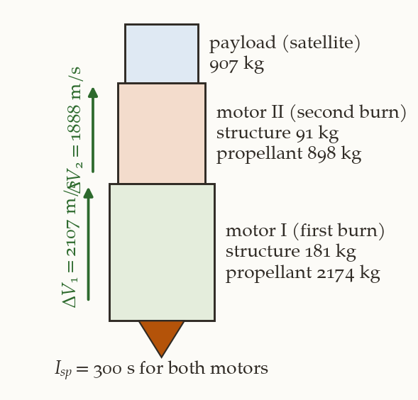
Most satellites delivered to low orbit by the Space Shuttle then reached their working orbit with a solid-propellant upper stage: an inertial upper stage (IUS) or a payload assist module (PAM) (Chobotov 2002). A solid motor is a case full of propellant with a nozzle. It burns until the propellant is gone. It cannot be throttled; in practice it cannot be stopped or restarted. A transfer between two orbits usually needs two burns, so the upper stage is two solid motors in a stack (Figure 1): stage I fires first, stage II second.
Each motor changes the velocity by an amount fixed by the rocket equation of the first chapter. Let us derive it again, because it fixes the meaning of the symbols. A rocket of mass \(m\) ejects a small mass \(-\mathrm dm>0\) backwards at the exhaust speed \(u\) relative to itself. Momentum conservation for the rocket and the ejected gas (no external force) gives \(m\,\mathrm dv=-u\,\mathrm dm\), so \(\mathrm dv=-u\,\mathrm dm/m\). Integrating from the initial mass \(m_i\) to the final mass \(m_f\) (with \(u\) constant),
\[ \Delta V=u\ln\frac{m_i}{m_f},\qquad u=g_0I_{sp},\qquad\text{i.e.}\qquad \frac{W_i}{W_f}=\exp\Bigl(\frac{\Delta V}{g_0I_{sp}}\Bigr) , \tag{1}\]
where \(I_{sp}\) is the specific impulse (in seconds), \(g_0=9.80665\) m/s\(^2\) the standard gravity that defines \(I_{sp}\) in seconds, and \(W=mg_0\) the weight at the Earth’s surface. The ratio \(W_i/W_f\) equals \(m_i/m_f\), which is why the book can use weights or masses: only the ratio matters. This is Chobotov’s (6.1).
A motor has \(I_{sp}=300\) s and burns from \(W_i=1896\) kg to \(W_f=998\) kg. What is its \(\Delta V\)?
What you should find
\(W_i/W_f=1.8998\), \(\ln1.8998=0.6416\), and \(\Delta V=9.80665\times300\times0.6416=1888.0\) m/s. (This is the second motor of the example below.)Because the motor cannot be stopped, the two \(\Delta V\)s of the upper stage are numbers given by the hardware, \(\Delta V_1\) and \(\Delta V_2\). The transfer has to use exactly these. This is the velocity-matching (or fixed-impulse) problem (Chu, Lang, and Winn 1978). Two cases are trivial: if \(\Delta V_1+\Delta V_2\) is less than the total of the best transfer, nothing can be done, the satellite cannot reach its orbit. If it is more, the stage has excess energy, and the excess has to go somewhere. That is the complication.
Three things the book does not say. (i) The motors are impulsive: their burn time is neglected, so the \(\Delta V\) of each is applied at one point; section 3 relaxes this. (ii) The two burns are at the ends of the transfer orbit’s major axis (perigee and apogee, as in a Hohmann transfer), at least until the book relaxes it; the plane change at each burn is made by turning the thrust out of the orbit plane. (iii) The initial and final orbits are circular. Everything below depends on them.
2.2 Ways to use up the excess
A designer who has fixed motors and a mission whose optimal \(\Delta V\) is less than the motors give can:
- Offload propellant: remove some from the motor. This is costly, and for a large offload the motor may have to be requalified for flight.
- Add ballast: put dead weight on the stage, which lowers its \(\Delta V\) through the rocket equation. Once the second stage matches, the first may be left without enough, and bolting weights to the payload invalidates tests already made.
- Modify the trajectory: change the transfer so that it needs more \(\Delta V\) than the optimal one. The excess is used on an extra plane change, an extra altitude change, an extra flight-path-angle change. Usually there is not one solution but a range, which can be exploited, as we shall see, to get a launch window.
Chobotov develops the third. We follow him with the example of his text.
2.3 The example: a Shuttle-delivered navigation satellite
A constellation of satellites is in circular orbits with a \(12\)-h period, at the height \(h_2=20\,187\) km and the inclination \(i_2=55^\circ\). A satellite is delivered by the Shuttle to a circular parking orbit at \(h_1=278\) km, at an inclination \(i_1\) that we are free to choose within limits, and is then carried up by two solid motors. The motors are (Figure 1, with Chobotov’s weights):
| structure | propellant | |
|---|---|---|
| payload (satellite) | \(907\) kg | |
| motor II (second burn) | \(91\) kg | \(898\) kg |
| motor I (first burn) | \(181\) kg | \(2174\) kg |
At the second burn the stage is payload plus motor II: \(W_i=907+91+898=1896\) kg before, \(W_f=907+91=998\) kg after (the propellant is gone, the structure stays). At the first burn the stage is everything: \(W_i=907+91+898+181+2174=4251\) kg before, and after burnout of motor I it is payload plus motor II plus motor I’s empty case, \(W_f=907+91+898+181=2077\) kg. Then
\[ \Delta V_2=9.80665\times300\ln\frac{1896}{998}=1888.0\ \text{m/s},\qquad \Delta V_1=9.80665\times300\ln\frac{4251}{2077}=2107.1\ \text{m/s}, \]
as in the book (\(1888\) and \(2107\) m/s).
Plain Hohmann transfer. First what the transfer would cost with no plane change. The radii are \(r_1=6378.137+278=6656.137\) km and \(r_2=6378.137+20\,187=26\,565.137\) km. The circular speeds are \(V_{c1}=\sqrt{\mu/r_1}=7738.5\) m/s and \(V_{c2}=\sqrt{\mu/r_2}=3873.6\) m/s. The transfer ellipse has \(a_{TR}=(r_1+r_2)/2=16\,610.6\) km, and by the vis-viva equation \(V=\sqrt{\mu(2/r-1/a)}\) the speeds at its two ends are
\[ V_{PTR}=\sqrt{\mu\Bigl(\frac2{r_1}-\frac1{a_{TR}}\Bigr)}=9786.3\ \text{m/s},\qquad V_{ATR}=\sqrt{\mu\Bigl(\frac2{r_2}-\frac1{a_{TR}}\Bigr)}=2452.1\ \text{m/s}. \]
A Hohmann transfer would cost \(V_{PTR}-V_{c1}=2047.8\) m/s and \(V_{c2}-V_{ATR}=1421.5\) m/s, a total of \(3469.4\) m/s. The motors supply \(\Delta V_1+\Delta V_2=3995.2\) m/s. The excess is \(525.8\) m/s, and it has to be spent.
2.4 Spending the excess on a plane change
The simplest way: do a Hohmann-type transfer in which a plane change accompanies each burn. Turning the velocity vector out of the orbit plane costs \(\Delta V\) (Figure 2 (a)). At the first burn the velocity before is the circular velocity \(\mathbf V_{c1}\) (length \(V_{c1}\)); after the burn it must be the transfer velocity at perigee, length \(V_{PTR}\), in a direction rotated by the angle \(\alpha_1\) about the radius vector. The two vectors form a triangle with the angle \(\alpha_1\) between them, and the third side is the velocity change, so by the law of cosines
\[ \Delta V_1^{\,2}=V_{c1}^{\,2}+V_{PTR}^{\,2}-2V_{c1}V_{PTR}\cos\alpha_1 , \tag{2}\]
and in the same way at the apogee
\[ \Delta V_2^{\,2}=V_{c2}^{\,2}+V_{ATR}^{\,2}-2V_{c2}V_{ATR}\cos\alpha_2 . \tag{3}\]
(These are Chobotov’s (6.3) and (6.2).) Here is the algebra behind the picture, which the book skips. Put the radius vector along the \(z\) axis. The two velocities are both horizontal (perpendicular to \(z\)): \(\mathbf V_{c}=(V_c,0,0)\) before, and \(\mathbf V_{t}=V_t(\cos\alpha,\sin\alpha,0)\) after, the transfer-orbit velocity turned by \(\alpha\) about the radius vector. Then \(|\mathbf V_t-\mathbf V_c|^2=V_t^2+V_c^2-2V_cV_t\cos\alpha\). Note that \(\alpha\) is the angle by which the orbit plane tilts: the orbit plane is the plane containing the radius vector and the velocity, and rotating the velocity about the radius vector by \(\alpha\) rotates the plane by the same angle \(\alpha\) about the same axis. (This is also checked numerically in the script.)
Equations (Equation 2) and (Equation 3) are now solved for the angles, given the fixed \(\Delta V\)s:
\[ \cos\alpha_1=\frac{V_{c1}^{\,2}+V_{PTR}^{\,2}-\Delta V_1^{\,2}}{2V_{c1}V_{PTR}},\qquad \cos\alpha_2=\frac{V_{c2}^{\,2}+V_{ATR}^{\,2}-\Delta V_2^{\,2}}{2V_{c2}V_{ATR}} . \tag{4}\]
Inserting the numbers, with the speeds in km/s (\(V_{c1}=7.7385\), \(V_{PTR}=9.7863\), \(\Delta V_1=2.1071\); \(V_{c2}=3.8736\), \(V_{ATR}=2.4521\), \(\Delta V_2=1.8880\)):
\[ \cos\alpha_1=\frac{59.883+95.772-4.440}{2(7.7385)(9.7863)}=0.99838,\quad \alpha_1=3.27^\circ;\qquad \cos\alpha_2=\frac{15.005+6.013-3.565}{2(3.8736)(2.4521)}=0.9187,\quad \alpha_2=23.26^\circ , \]
the book’s \(3.25^\circ\) and \(23.25^\circ\). So the motors are exactly used up if the first burn tilts the plane by \(3.27^\circ\) and the second by \(23.26^\circ\): the second burn, where the speed is low, takes most of the plane change, as it should be, because a plane change is cheapest where the speed is lowest.
How good a choice is the split \(3.27^\circ\) / \(23.26^\circ\), from the point of view of fuel? Suppose we wanted the total plane change \(26.53^\circ\) at the lowest total \(\Delta V\), and the motors were not fixed: how would the best split compare?
Answer
Minimise \(\Delta V_1+\Delta V_2\) over \(\alpha_1\) with \(\alpha_1+\alpha_2=26.53^\circ\) held fixed: the minimum is at \(\alpha_1=3.17^\circ\) and costs \(3995.11\) m/s. The motors, forced to \(3.27^\circ\), cost \(3995.16\) m/s: \(0.05\) m/s more. The fixed motors happen to deliver almost exactly the best possible split. (Doing the whole \(26.53^\circ\) at the apogee burn would cost \(4053.0\) m/s, \(58\) m/s more.) The designer’s motors were evidently chosen for this transfer.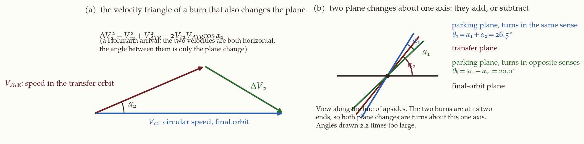
2.5 How far apart can the parking orbit and the final orbit be?
What the motors fixed is \(\alpha_1\) and \(\alpha_2\). What we need to know is which parking orbits the Shuttle can be in. A parking orbit is characterised by its inclination \(i_1\) and the right ascension of its ascending node \(\Omega_1\), and what matters is how far it is from the final orbit, in two numbers: the angle \(\theta\) between the two orbit planes, which this section computes, and the difference of nodes \(\Delta\Omega=\Omega_1-\Omega_2\), which the next one will relate to the launch time.
The total plane change. Both burns of a Hohmann-type transfer are at the two ends of the same straight line (the line of apsides). The first rotates the orbit plane by \(\alpha_1\) about this line; the second by \(\alpha_2\) about the same line. Two rotations about one axis simply add their angles when made in the same sense, and subtract when made in opposite senses (Figure 2 (b)). The total angle \(\theta\) between the parking orbit and the final orbit is therefore
\[ \theta_a=\alpha_1+\alpha_2=26.53^\circ\ \ (\text{same sense}),\qquad \theta_b=|\alpha_1-\alpha_2|=19.99^\circ\ \ (\text{opposite senses}) , \tag{5}\]
(Chobotov’s \(26.5^\circ\) and \(20^\circ\)). The Shuttle’s parking orbit may be at either of two angles from the final orbit; the transfer is made in the sense that gives the angle in question.
The relation of \(\theta\) to the inclination and the node. Each orbit plane has a unit normal, \(\hat{\mathbf n}=(\sin i\sin\Omega,\ -\sin i\cos\Omega,\ \cos i)\) (the direction of the angular momentum; check: for \(i=0\) it is the \(z\) axis). The angle between two planes is the angle between their normals, so \(\cos\theta=\hat{\mathbf n}_1\cdot\hat{\mathbf n}_2\):
\[ \boxed{\cos\theta=\cos i_1\cos i_2+\sin i_1\sin i_2\cos\Delta\Omega} \tag{6}\]
(Chobotov’s (6.4); the product is expanded in the script by symbolic algebra.) This is the spherical law of cosines for the triangle formed by the pole and the two normals.
The special case \(\Delta\Omega=0\), parking and final orbits with the same node: then \(\theta=|i_1-i_2|\), and the plane change is purely an inclination change, so the parking inclinations are \(i_1=i_2\pm\theta\). With \(i_2=55^\circ\):
\[ i_1=55^\circ\pm26.53^\circ=28.47^\circ\ \text{or}\ 81.53^\circ,\qquad i_1=55^\circ\pm19.99^\circ=35.01^\circ\ \text{or}\ 74.99^\circ , \]
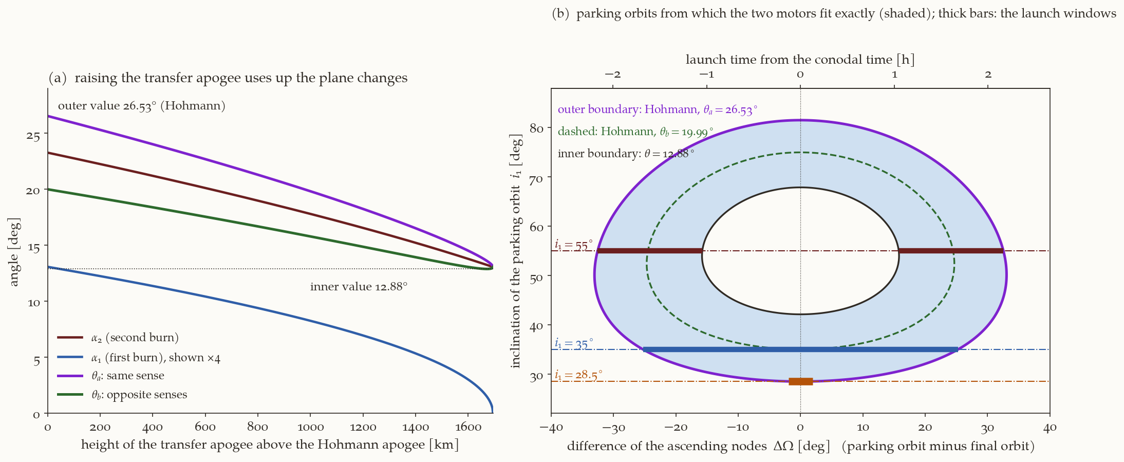
the book’s \(28.5^\circ\), \(81.5^\circ\), \(35^\circ\), \(75^\circ\). A Shuttle orbit at one of those four inclinations, with the right node, is served by the Hohmann transfer of the motors. In general the Shuttle orbit does not have to have the same node as the final orbit, and then (Equation 6) gives, for each \(i_1\), the node difference \(\Delta\Omega\) that makes the angle equal to \(\theta_a\) (or \(\theta_b\)): \(\cos\Delta\Omega=(\cos\theta-\cos i_1\cos i_2)/(\sin i_1\sin i_2)\). Plotting \(\Delta\Omega\) against \(i_1\) for \(\theta=\theta_a\) and for \(\theta=\theta_b\) gives the two closed curves of Chobotov’s Fig. 6.5, which are the loci of parking orbits that match \(\Delta V_1\) and \(\Delta V_2\) with Hohmann transfers; the outer one is the purple curve of Figure 3 (b) and the dashed green one inside it is \(\theta_b\).
2.6 Non-Hohmann transfers: using up the excess in a different way
There is nothing sacred about the Hohmann transfer. Suppose the apogee of the transfer orbit is raised above the final orbit, so that the transfer ellipse crosses the final circle at the second burn instead of touching it (Chobotov’s Fig. 6.6). Three things change.
- The perigee speed \(V_{PTR}\) rises (a larger ellipse). With \(\Delta V_1\) fixed, Equation 2 then allows less plane change: \(\alpha_1\) decreases, until at \(V_{PTR}=V_{c1}+\Delta V_1\) it is zero (the whole \(\Delta V_1\) is needed for the speed change).
- At the crossing the transfer velocity has a flight-path angle \(\gamma_2\): it is not horizontal, it points outward (on the way up) or inward (on the way down). The circular velocity of the final orbit is horizontal, so the velocity change at the second burn must now remove the flight-path angle as well as the plane angle. The velocity after the burn is horizontal and in the final plane: \(\mathbf V_c=(V_{c2},0,0)\). The transfer velocity before the burn is \(\mathbf V_t=V_t(\cos\gamma_2\cos\alpha_2,\ \cos\gamma_2\sin\alpha_2,\ \sin\gamma_2)\): horizontal components rotated by \(\alpha_2\), and a radial component \(V_t\sin\gamma_2\). Then \[ \Delta V_2^{\,2}=|\mathbf V_t-\mathbf V_c|^2=V_{c2}^{\,2}+V_t^{\,2}-2V_{c2}V_t\cos\gamma_2\cos\alpha_2 , \tag{7}\] which reduces to Equation 3 for \(\gamma_2=0\) (the proof is in the script, symbolically). Since \(\cos\gamma_2<1\), the same \(\Delta V_2\) gives a smaller \(\alpha_2\): \(\alpha_2\) decreases.
- The two burns are no longer at opposite ends of the line of apsides: the second is at the true anomaly \(f_2<180^\circ\) of the transfer orbit (the crossing on the way up) or at \(360^\circ-f_2\) (on the way down). The two plane changes are rotations about two different radius vectors, and the angles no longer simply add. Chobotov remarks that \(\theta_a\) and \(\theta_b\) “are no longer the simple sum and difference” and refers to the literature (Chu, Lang, and Winn 1978). Here is the result.
The composition of two plane changes about different axes. Let \(\hat{\mathbf n}_t\) be the normal of the transfer plane. The final plane is the transfer plane turned about the radius vector \(\hat{\mathbf e}_2\) of the second burn by \(\alpha_2\), and the parking plane is the transfer plane turned about the radius vector \(\hat{\mathbf e}_1\) of the first burn by \(\alpha_1\). Both \(\hat{\mathbf e}_1\) and \(\hat{\mathbf e}_2\) lie in the transfer plane, with the angle \(f_2\) between them (the true anomaly of the second burn, counted from the perigee, where the first is). A rotation of \(\hat{\mathbf n}_t\) about an axis in the plane perpendicular to it by the angle \(\alpha\) gives \(\hat{\mathbf n}=\hat{\mathbf n}_t\cos\alpha\pm\hat{\mathbf p}\sin\alpha\), where \(\hat{\mathbf p}=\hat{\mathbf e}\times\hat{\mathbf n}_t\) is a unit vector in the transfer plane, perpendicular to the axis, and the sign gives the sense. The vectors \(\hat{\mathbf p}_1\) and \(\hat{\mathbf p}_2\) are the vectors \(\hat{\mathbf e}_1\), \(\hat{\mathbf e}_2\) both turned by \(90^\circ\) about \(\hat{\mathbf n}_t\), so the angle between them is also \(f_2\), and \(\hat{\mathbf p}_1\cdot\hat{\mathbf p}_2=\cos f_2\). The angle between the parking and the final orbit planes is then given by
\[ \boxed{\cos\theta=\hat{\mathbf n}_1\cdot\hat{\mathbf n}_2=\cos\alpha_1\cos\alpha_2\pm\sin\alpha_1\sin\alpha_2\cos f_2} \tag{8}\]
(the dot products \(\hat{\mathbf n}_t\cdot\hat{\mathbf p}\) vanish; the script checks this on \(600\) random configurations). For \(f_2=180^\circ\) this is \(\cos(\alpha_1\mp\alpha_2)\): the Hohmann result Equation 5 is the special case. For \(f_2<180^\circ\) the two angles \(\theta_a\) (the \(+\) sign) and \(\theta_b\) (the \(-\) sign) come closer together. The ascending and the descending crossing have the same \(\cos f_2\), so the same angles; they differ in the flight time, which is why the book calls the two end cases “max/min flight time” transfers.
Numbers. Table 3 lists the family. As the apogee is raised, both \(\alpha_1\) and \(\alpha_2\) fall and the angles \(\theta_a\) and \(\theta_b\) close in on each other. The family stops where \(\alpha_1\) reaches zero, \(V_{PTR}=V_{c1}+\Delta V_1=9845.7\) m/s, which is an apogee radius of \(28\,259\) km, only \(1694\) km above the Hohmann apogee (Figure 3 (a)): a big increase of the apogee would need much more \(\Delta V_1\) than the motors have. At the end of the family the second burn removes a flight-path angle of \(\gamma_2=22.95^\circ\) and a plane change of \(\alpha_2=13.06^\circ\).
| apogee above the Hohmann one [km] | \(\alpha_1\) | \(\alpha_2\) | \(\gamma_2\) | \(f_2\) | \(\theta_a\) | \(\theta_b\) |
|---|---|---|---|---|---|---|
| \(0\) (Hohmann) | \(3.27^\circ\) | \(23.26^\circ\) | \(0^\circ\) | \(180.0^\circ\) | \(26.53^\circ\) | \(19.99^\circ\) |
| \(100\) | \(3.17^\circ\) | \(22.75^\circ\) | \(6.05^\circ\) | \(175.9^\circ\) | \(25.91^\circ\) | \(19.60^\circ\) |
| \(500\) | \(2.73^\circ\) | \(20.66^\circ\) | \(13.23^\circ\) | \(171.0^\circ\) | \(23.35^\circ\) | \(17.97^\circ\) |
| \(1000\) | \(2.07^\circ\) | \(17.79^\circ\) | \(18.23^\circ\) | \(167.4^\circ\) | \(19.81^\circ\) | \(15.79^\circ\) |
| \(1694\) (limit, \(\alpha_1=0\)) | \(0\) | \(13.06^\circ\) | \(22.95^\circ\) | \(163.9^\circ\) | \(13.06^\circ\) | \(13.06^\circ\) |
The region. For each member of the family there is a locus of parking orbits, from which the transfer can be flown with the exact \(\Delta V_1\) and \(\Delta V_2\): the curves \(\theta=\theta_a\) and \(\theta=\theta_b\) of that member, in the plane of \((\Delta\Omega,i_1)\) of Equation 6. All members together fill the region between the outer curve \(\theta=26.53^\circ\) (the Hohmann transfer, with the largest total plane change) and the inner curve \(\theta=12.88^\circ\) (the smallest \(\theta\) of any member, near the end of the family); this is Chobotov’s Fig. 6.8, redrawn in Figure 3 (b). Points outside the outer curve are too far from the final orbit for the motors’ \(\Delta V\) to be enough; points inside the inner curve are too close, so that even the trajectory modification cannot absorb the excess energy. Inside the shaded region a parking orbit may have more than one transfer that uses the motors exactly.
2.7 Launch window
Chobotov observes that supplying excess energy buys something: a launch window, a stretch of time during which a ground launch to the Shuttle orbit is possible. The idea is simple once the region of Figure 3 (b) is known. A launch from the ground into an orbit of inclination \(i_1\) puts the orbit’s ascending node at a right ascension that depends on when the launch is made. The orbital plane of a launch is fixed in inertial space once the vehicle is in orbit, but the launch site is carried eastward by the Earth’s rotation at \(15.041^\circ\) per hour, so a launch \(t\) hours later than the one that gives the target plane puts the node \(15.041\,t\) degrees farther east:
\[ \Omega=\Omega_0+15\,t\quad(\text{degrees, }t\text{ in hours}), \tag{9}\]
where \(\Omega_0\) is the right ascension of the node that the target plane would have for a launch at \(t=0\). The book writes \(15\); \(360^\circ/23.9345\ \text{h}=15.041^\circ\)/h is the exact rotation against the stars. The launch time \(t=0\) at which the node of the Shuttle orbit equals the node of the final orbit (\(\Delta\Omega=0\)) is called the conodal launch time. So the node difference of the Shuttle orbit is \(\Delta\Omega=15.041\,t\), and the launch window for a Shuttle orbit of inclination \(i_1\) is read off Figure 3 (b) along the horizontal line \(i_1=\text{const}\): the stretch of \(\Delta\Omega\) inside the shaded region, divided by \(15.041^\circ\)/h.
- \(i_1=55^\circ\) (same inclination as the final orbit): the line cuts the shaded region in two stretches, \(15.75^\circ\le|\Delta\Omega|\le32.53^\circ\): two windows, \(1.05\) to \(2.16\) h before and after the conodal time, each about an hour long. Around \(t=0\) the Shuttle orbit is almost the final orbit (\(\theta\) near \(0\)), the motors have too much \(\Delta V\) for any trajectory modification, and the window is closed. (The book reads \(17^\circ\) to \(32^\circ\), \(1.13\) to \(2.13\) h, from his plot; the difference is the reading of the figure.)
- \(i_1=35^\circ\): the line goes through the region without a gap (the planes are \(20^\circ\) apart at \(\Delta\Omega=0\), inside the allowed band), \(|\Delta\Omega|\le25.27^\circ\): one window of \(\pm1.68\) h around the conodal time (the book: \(\pm1.73\) h).
- \(i_1=28.5^\circ\) (the launch latitude: the lowest inclination one can reach): the line touches the region only at its lowest point, \(|\Delta\Omega|\le1.9^\circ\), \(\pm7.7\) minutes: the book calls it “an instant”, the moment when the final orbit plane passes over the launch site.
Whenever the Shuttle launch falls inside the window, a transfer exists that consumes exactly the motors’ \(\Delta V\). The width of the window is a direct measure of how much room the excess energy gives.
Why is there no launch window close to the conodal time for the \(55^\circ\) Shuttle orbit, even though that is the time when the two planes coincide and one might expect the best transfer?
Answer
When the two planes coincide, the best transfer is the coplanar Hohmann transfer, which costs only \(3469\) m/s. The motors carry \(3995\) m/s. The surplus of \(526\) m/s cannot be spent: a plane change is the way to spend it, and when the planes already coincide there is nothing to change; raising the apogee does not help either (Table 3: the smallest total plane change of the family is \(12.88^\circ\)). The motors would put the satellite in the wrong orbit. The excess energy can be absorbed only if the parking orbit is tilted away from the final orbit by at least \(12.88^\circ\): that is why the window has a hole at the centre.2.8 The book’s problems 6.1 and 6.3, worked
Problem 6.1 (a heavier satellite). The payload mass of the example is raised from \(907\) kg to \(990\) kg on the same upper stage. (a) The \(\Delta V\)s are now \(\Delta V_2=9.80665\times300\ln\frac{990+91+898}{990+91}=1779.0\) m/s and \(\Delta V_1=9.80665\times300\ln\frac{990+91+898+181+2174}{990+91+898+181}=2048.8\) m/s. (b) The plain Hohmann transfer needs \(V_{PTR}-V_{c1}=2047.8\) m/s at the first burn: the motor delivers \(2048.8\) m/s, only \(0.9\) m/s more, so \(\cos\alpha_1=(V_{c1}^2+V_{PTR}^2-\Delta V_1^2)/(2V_{c1}V_{PTR})\) gives \(\alpha_1=0.41^\circ\) (the book: \(\approx0\)). And \(\alpha_2=19.99^\circ\) (book: \(19.97^\circ\)): the second motor takes all the plane change. (c) The loci are two curves, for \(\theta_a=20.39^\circ\) and \(\theta_b=19.58^\circ\), almost the single circle \(\theta=19.99^\circ\) (Equation 6, as before). (d) Non-Hohmann transfers: the first burn has \(0.9\) m/s of slack and, as we found, a higher apogee needs more \(\Delta V_1\): the apogee can rise by only \(25\) km. So the loci are essentially unchanged. The allowed locus does not grow. (e) For a Shuttle orbit at \(i_1=55^\circ\): \(\theta=20.39^\circ\) or \(19.58^\circ\) gives \(\Delta\Omega=24.96^\circ\) or \(23.96^\circ\), i.e. launch at \(1.66\) h or \(1.59\) h before or after the conodal time. The two loci are \(1.0^\circ\) apart, so the window is two pairs of windows about four minutes long: nearly instants. Less excess energy, narrower windows.
Problem 6.3 (two identical motors, a \(296\) km orbit to a \(741\) km orbit, highest possible inclination). The payload is \(1452\) kg; each motor has \(1044\) kg of propellant, \(136\) kg of structure and \(I_{sp}=285\) s. The highest Shuttle-orbit inclination allowed by range safety is \(57^\circ\); the experimenters want an orbit as steeply inclined as possible, preferably above \(72^\circ\).
Second burn: \(\Delta V_2=9.80665\times285\ln\frac{1452+136+1044}{1452+136}=1412.2\) m/s. First burn: \(\Delta V_1=9.80665\times285\ln\frac{1452+136+1044+136+1044}{1452+136+1044+136}=894.4\) m/s. (The book: \(894\), \(1412\).)
The Hohmann transfer between \(r_1=6674\) km and \(r_2=7119\) km (the book’s Earth radius \(6378\) km) has \(V_{c1}=7728.2\), \(V_{PTR}=7851.8\), \(V_{ATR}=7361.0\) and \(V_{c2}=7482.7\) m/s, so a tangential burn would need only \(123.7\) m/s at the first burn and \(121.7\) m/s at the second. The motors have \(894.4\) and \(1412.2\) m/s: almost all of it goes into plane change. Equation 4 gives \(\alpha_1=6.52^\circ\) and \(\alpha_2=10.88^\circ\).
The destination orbit can be inclined from the Shuttle orbit by \(\alpha_1+\alpha_2=17.40^\circ\) at most (both changes in the same sense), so \(i_{2,\max}=57^\circ+17.40^\circ=74.40^\circ>72^\circ\): the goal is met.
The transfer orbit is tilted by \(\alpha_1\) from the Shuttle orbit: \(i_{tr}=57^\circ+6.52^\circ=63.52^\circ\). Both plane changes are pure inclination changes (the node does not change), so they are made at the nodes: the burns are at the equator, at latitude \(0^\circ\), the first at one node and the second at the opposite one (\(180^\circ\) later).
3 Finite-duration burns: gravity losses
3.1 The equation of motion of a rocket in a gravity field
Every \(\Delta V\) so far was applied in no time at all. A real engine has a thrust \(T\) that is finite, and the thrust-to-weight ratio \(T/W\) (here and below \(W_0\) is the weight at ignition) is in practice between \(10^{-5}\) and \(10\). A burn of a few minutes covers a good arc of the orbit, and during it gravity keeps changing the velocity. To see by how much, we write the equation of motion of the rocket along its flight path, with the thrust along the velocity.
Take a rocket of mass \(m\) and speed \(V\) (we write the speed as \(V\) in this section; the book writes \(v\)). The exhaust leaves with the speed \(u\) relative to the rocket. The momentum balance for a rocket under an external force \(F\) along its direction of motion follows from comparing the momentum at \(t\) and at \(t+\mathrm dt\). At \(t\) the rocket has mass \(m\) and speed \(V\): momentum \(mV\). At \(t+\mathrm dt\) the rocket has mass \(m+\mathrm dm\) (with \(\mathrm dm<0\)) and speed \(V+\mathrm dV\), and the gas \(-\mathrm dm>0\) that it ejected has the speed \(V-u\) (the exhaust speed \(u\) is relative to the rocket, backwards). The change of the total momentum is the impulse of the external force:
\[ (m+\mathrm dm)(V+\mathrm dV)+(-\mathrm dm)(V-u)-mV=F\,\mathrm dt . \]
Expanding, \(m\,\mathrm dV+V\,\mathrm dm+\mathrm dm\,\mathrm dV-V\,\mathrm dm+u\,\mathrm dm=F\,\mathrm dt\); the terms \(V\,\mathrm dm\) cancel, and the product \(\mathrm dm\,\mathrm dV\) is of second order and is dropped, so \(m\,\mathrm dV+u\,\mathrm dm=F\,\mathrm dt\), that is
\[ m\frac{\mathrm dV}{\mathrm dt}=-u\frac{\mathrm dm}{\mathrm dt}+F . \]
The first term is the thrust \(T=-u\,\dot m=g_0I_{sp}\,|\dot m|\) (positive because \(\dot m<0\)). The external forces are, along the velocity, the drag \(D\) (opposing the motion) and the component of the weight \(mg\) along the flight path. If \(\gamma\) is the angle of the flight path above the local horizontal, the weight points toward the centre of the Earth, which is at the angle \(90^\circ+\gamma\) from the velocity, so its component along the velocity is \(-mg\sin\gamma\). Hence \(F=-D-mg\sin\gamma\):
\[ m\frac{\mathrm dV}{\mathrm dt}=-u\frac{\mathrm dm}{\mathrm dt}-D-mg\sin\gamma . \]
Multiply by \(\mathrm dt/m\):
\[ \mathrm dV=-u\frac{\mathrm dm}{m}-\frac Dm\,\mathrm dt-g\sin\gamma\,\mathrm dt . \]
Integrate over the burn, from the initial mass \(m_i\) to the final mass \(m_f\) (the first term is \(u\ln(m_i/m_f)\), as in Equation 1):
\[ \boxed{\Delta V=g_0I_{sp}\ln\frac{m_i}{m_f}-\int\frac Dm\,\mathrm dt-\int g\sin\gamma\,\mathrm dt} \tag{10}\]
(Chobotov’s (6.5).) The left side is the change of speed that the burn actually produces. The first term on the right is the ideal rocket-equation \(\Delta V\). The other two are losses: the drag loss (zero above the atmosphere, which we assume from now on) and the gravity loss \(\int g\sin\gamma\,\mathrm dt\). The sum \(\int g\sin\gamma\,\mathrm dt\) is positive when the vehicle is climbing (\(\gamma>0\)): gravity is then slowing it down, and the engine has to make up for that. When the vehicle descends (\(\gamma<0\)) the integrand is negative, and gravity is helping.
Four things in (Equation 10). (i) The thrust is along the velocity (a “tangential” burn): otherwise there would be a steering term. (ii) \(\Delta V\) is a scalar speed change along the path, not a vector change: a burn also turns the velocity, and the turning is not counted. (iii) \(g\) is the local gravitational acceleration, which changes as the vehicle climbs. (iv) For a burn from the ground \(\gamma\) is the angle between the flight path and the horizontal; for a burn in orbit it is the same angle, the flight-path angle of the orbit’s velocity.
3.2 The simplest case: a vertical ascent
If the burn is vertical, \(\gamma=90^\circ\), and with constant \(g\) (a short burn) the gravity loss is exactly \(g\,t_b\) with \(t_b\) the burn time. The burn time follows from the mass flow: constant thrust \(T\) gives \(\dot m=T/u\), so the mass falls from \(m_0\) to \(m_f=m_0/R\) in \(t_b=(m_0-m_f)u/T=(1-1/R)\,u/(T/m_0)\). With \(T/m_0=(T/W_0)\,g\),
\[ \text{loss}=g\,t_b=\frac{u\,(1-1/R)}{T/W_0}\ ,\qquad \Delta V=u\Bigl[\ln R-\frac{1-1/R}{T/W_0}\Bigr] ,\qquad R=\frac{m_0}{m_f} . \tag{11}\]
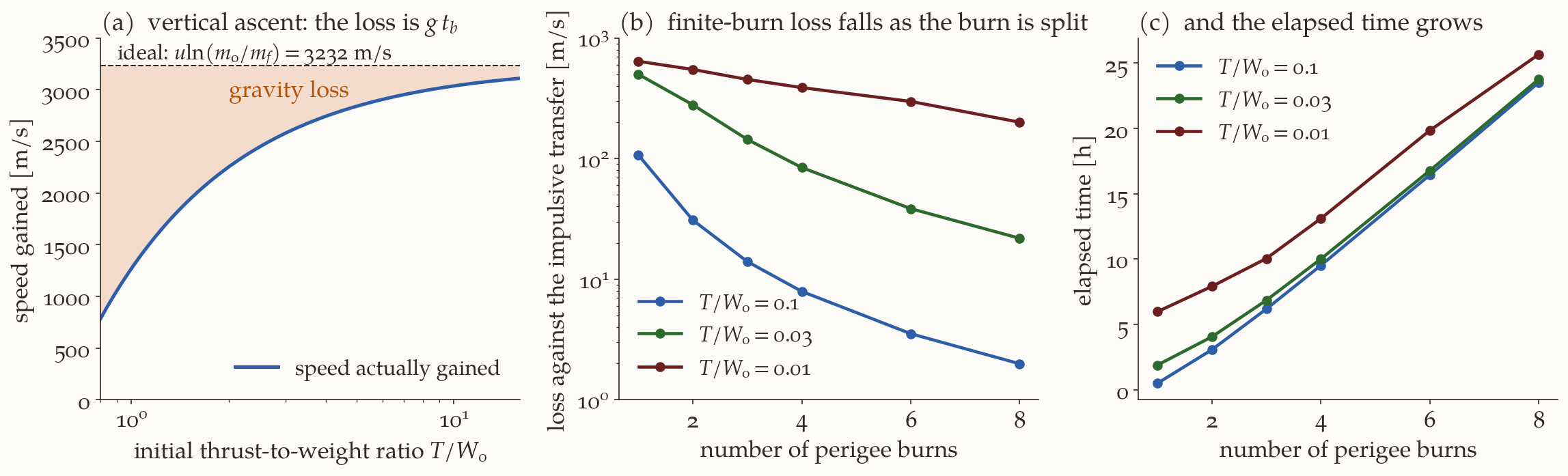
So the loss is inversely proportional to the thrust-to-weight ratio: double the thrust, halve the loss (Figure 4 (a)). With \(I_{sp}=300\) s and \(R=3\) (\(m_f=m_0/3\)): the ideal \(\Delta V\) is \(u\ln R=3232\) m/s. At \(T/W_0=1.5\) the loss is \(1308\) m/s and the vehicle gains \(1925\) m/s; at \(T/W_0=3\) the loss is \(654\) m/s. Integrating the equation of motion numerically reproduces this to the last digit (the script). This is why launch vehicles have \(T/W_0\) of order \(1.2\) to \(1.5\) at lift-off: it must exceed \(1\) for the vehicle to leave the pad at all, a value close to \(1\) wastes \(\Delta V\) on gravity, and a much higher value needs a heavier engine and structure.
3.3 Gravity loss in orbit, and what drives it
For an orbital burn the same equation holds, with \(\gamma\) now the flight-path angle of the orbit. Chobotov lists three factors that raise the loss: a long burn (low thrust-to-weight ratio), high \(g\) (a burn at low altitude), and a large \(\gamma\) (a burn over a large central angle). The first two are visible in (Equation 10): the integral grows with the duration \(\mathrm dt\) and the factor \(g\). The third needs an explanation.
A Hohmann burn is impulsive and at perigee, where \(\gamma=0\). A finite burn surrounds the perigee: it starts before it, with the vehicle descending (\(\gamma<0\)), and ends after it, with the vehicle climbing (\(\gamma>0\)), and if the thrust is along the velocity the angle \(\gamma\) sweeps a range of about the size of the central angle covered. The book writes (its Fig. 6.11) that if the burn keeps the impulsive direction, the values of \(\gamma\) at the start and the end are about minus and plus the central angles \(\phi_1\), \(\phi_2\) swept before and after the impulsive point: near the middle of the burn \(\gamma\approx0\) and the contribution is nothing, but at the ends the \(\sin\gamma\) term is significant. This is a heuristic. To make it concrete, here is an exact numerical example, a burn of the type the next section uses. A vehicle on a \(278\) km orbit has already raised its apogee halfway to the geosynchronous radius (equal shares of the perigee-speed gain); its second perigee burn has \(T/W_0=0.1\) and \(I_{sp}=300\) s and is started half its duration before perigee, so as to be centred on it; the thrust is along the velocity, and it ends when the apogee reaches \(42\,164\) km. The numerical integration gives
- burn duration \(11.2\) min; \(\gamma\) runs from \(-6.17^\circ\) at the start to \(+11.13^\circ\) at the end (it crosses zero at the lowest point of the path, about \(0.4\) of the way through);
- ideal \(\Delta V=u\ln(m_i/m_f)=1231.9\) m/s; gravity integral \(\int g\sin\gamma\,\mathrm dt=152.6\) m/s; the speed actually gained is \(1079.3\) m/s, and \(1231.9-152.6=1079.3\): Equation 10 holds (to \(10^{-9}\) m/s in the script).
So for a burn of only \(11\) minutes at \(T/W_0=0.1\), \(12\%\) of the ideal \(\Delta V\) is spent climbing. And the integral is not zero even though \(\gamma\) changes sign: the vehicle is higher at the end than at the start (\(6934.8\) km to \(7130.2\) km), and the net effect of descending in the first part and climbing in the second is a net climb.
What is the effect on what we are after, the orbit’s energy? The energy of the orbit changes only because of the thrust, \(\mathrm d\varepsilon=\mathbf V\cdot\mathbf a_T\,\mathrm dt=V\,\mathrm d(\Delta V_{\rm ideal})\): every metre per second delivered at speed \(V\) raises the energy by \(V\), and the faster, the better (the Oberth effect). An impulsive burn at perigee delivers all its \(\Delta V\) at the highest speed of the orbit. A finite burn delivers part of it after the vehicle has climbed and slowed down, at a lower speed, so each metre per second buys less energy. In the example the energy gained is \(11.541\) km\(^2\)/s\(^2\) (the integral of \(V\,\mathrm d\Delta V\) equals the energy gain: checked in the script), \(1.0\%\) less than the \(11.664\) km\(^2\)/s\(^2\) that the same ideal \(\Delta V\) would give at the perigee speed. The shortfall of \(0.123\) km\(^2\)/s\(^2\) divided by the perigee speed (\(8.85\) km/s) is about \(14\) m/s: the engine has to supply that much additionally. (The two ways of counting the loss, \(153\) m/s of speed lost to climbing and \(14\) m/s of energy shortfall, measure different things: the first is the bookkeeping of the speed in Equation 10; the second is what the orbit energy gains. The same burn has both.)
3.4 The cure: several perigee burns
The obvious cure is a stronger engine. There is another one: break one long burn into several shorter ones, made at successive perigee passages. The vehicle is left in an orbit that is a little larger than before; after one revolution it is back at (nearly) the same perigee, and burns again. Each burn covers a smaller central angle, so the range of \(\gamma\) is smaller, the climb is smaller, and the loss is smaller: the second term in (Equation 10) is reduced. Chobotov’s Fig. 6.12 and 6.13 show the effect for a transfer from LEO (\(278\) km, \(28.5^\circ\)) to GEO; the \(\Delta V\) approaches the impulsive value (\(4237\) m/s) for high thrust, and the saving from splitting is “substantial”, paid for by transfer time.
To see the numbers ourselves, here is a clean experiment of our own (not Chobotov’s data, which are only in his plots). The model: a \(278\) km circular orbit; the goal is an orbit with apogee at the geosynchronous radius (\(r=42\,164\) km); the thrust is along the velocity and constant, \(I_{sp}=300\) s; the burn is divided into \(N\) burns of equal perigee-speed increments, each burn starts half its duration before the perigee so that it is centred on it, and each burn ends when the osculating apogee reaches its target. The engine \(\Delta V\) is the sum of \(u\ln(m_i/m_f)\) over the burns. To measure the loss, we compare with the cheapest impulsive transfer to the same final orbit (a long burn also raises the perigee, so the final orbit is not exactly the Hohmann ellipse): a Hohmann-type apogee raise at \(278\) km followed by a perigee raise at the apogee.
| \(T/W_0\) | \(N=1\) | \(N=2\) | \(N=4\) | \(N=8\) |
|---|---|---|---|---|
| \(0.1\) | \(107.0\) m/s, \(0.5\) h | \(30.9\) m/s, \(3.1\) h | \(7.9\) m/s, \(9.5\) h | \(2.0\) m/s, \(23.5\) h |
| \(0.03\) | \(499.8\) m/s, \(1.9\) h | \(278.9\) m/s, \(4.0\) h | \(84.2\) m/s, \(10.0\) h | \(21.8\) m/s, \(23.8\) h |
| \(0.01\) | \(640.3\) m/s, \(6.0\) h | \(547.9\) m/s, \(7.9\) h | \(387.6\) m/s, \(13.1\) h | \(200.2\) m/s, \(25.7\) h |
The picture (Figure 4 (b), (c)) is the one of the book: more burns, less loss, more time. Compare the two ways of reducing the loss at \(T/W_0=0.03\): either multiply the thrust by \(3.3\) (\(T/W_0=0.1\), one burn: \(107\) m/s) or split into eight burns (\(21.8\) m/s, but \(24\) h instead of \(1.9\) h). The tradeoff is the designer’s to make.
Three regimes. Chobotov divides the problem by thrust level.
- High thrust, \(T/W_0\gtrsim0.5\) to \(1\): the burn is short, the loss is a few m/s or tens of m/s (our \(1.2\) m/s at \(T/W_0=1\)), and the impulsive model is adequate, or one can correct it with Robbins’s analysis of the impulsive approximation (cited in the book).
- Low thrust, \(T/W_0\approx0.01\) to \(0.1\): thrust and gravity are comparable, estimates are unreliable, and “the best method of solution is to run an integrated trajectory computer program”. That is exactly what the experiment above is.
- Very low thrust, \(T/W_0\approx10^{-5}\): the thrust is a perturbation of the orbit, and the transfer is many revolutions of a slowly growing spiral. The next section treats it analytically.
4 Very low thrust transfers
4.1 Setting up
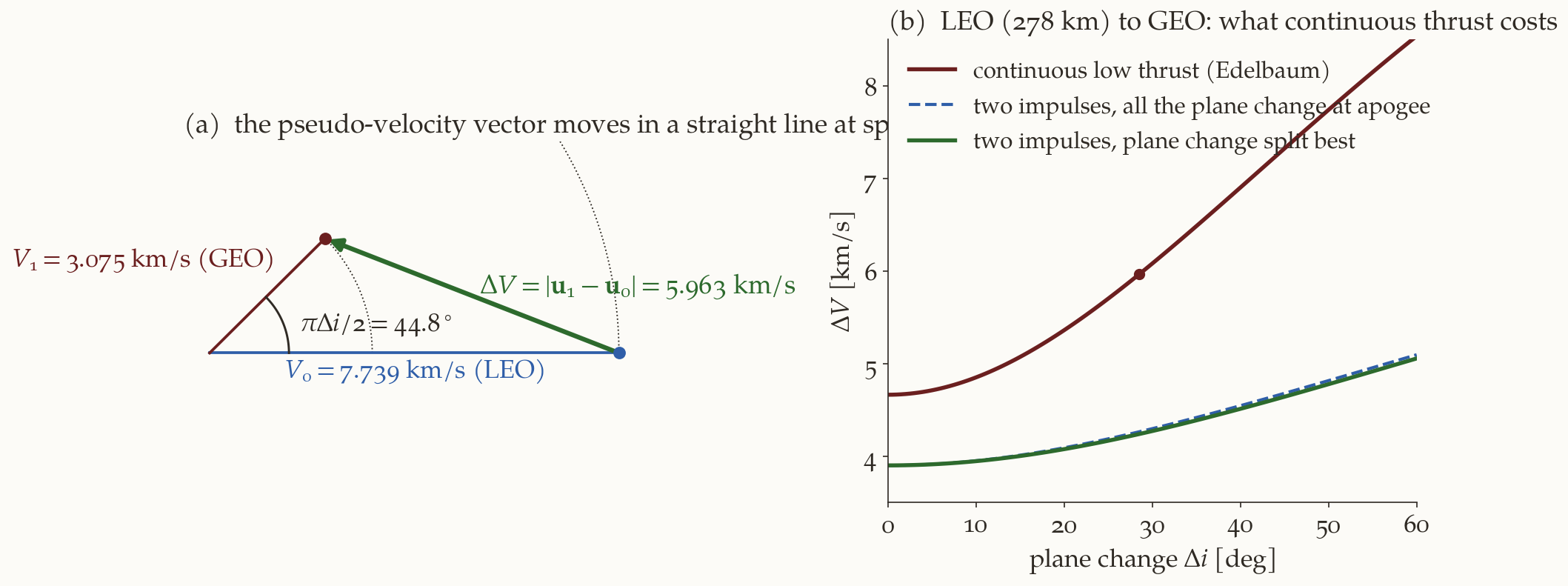
Electric propulsion accelerates at \(10^{-5}\) of the weight or so. Its specific impulse is high (thousands of seconds), so it uses very little propellant, but it takes weeks to do what a chemical stage does in minutes. The orbit is almost circular at every instant: each revolution is a slightly larger circle (and, if a plane change is wanted, a slightly different plane). Edelbaum (Edelbaum 1961) found a first-order analytic solution for the transfer between two circular orbits, with a change of plane of \(\alpha\) (the angle between the planes, in radians), which Chobotov reports:
\[ \boxed{\Delta V=\sqrt{V_0^{\,2}-2V_0V_1\cos\Bigl(\frac\pi2\alpha\Bigr)+V_1^{\,2}}} \tag{12}\]
where \(V_0\) and \(V_1\) are the circular speeds of the initial and the final orbit. The structure is the law of cosines again, but with the angle \(\frac\pi2\alpha\) instead of \(\alpha\). We now derive it, since the book only quotes it.
4.2 Derivation by a pseudo-velocity vector
Let the thrust acceleration have the constant magnitude \(a=T/m\) (to first order; mass changes are accounted for afterwards). Let it make the angle \(\beta\) with the velocity, in the plane that contains the velocity and the orbit normal, so that the tangential component is \(a\cos\beta\) and the normal one \(a\sin\beta\). Averaged over one revolution (this is where “very low thrust” is used: the orbit changes little in a revolution), the circular orbit evolves as follows.
- Speed. For a circular orbit \(V=\sqrt{\mu/r}\); a tangential acceleration \(a_t\) changes the energy at the rate \(\dot\varepsilon=Va_t\), and \(\varepsilon=-\mu/(2r)=-V^2/2\), so \(\dot\varepsilon=-V\dot V\), which gives \(\dot V=-a_t\). The speed decreases when the vehicle is accelerated tangentially: the orbit grows and its circular speed falls (the paradox of low-thrust spirals). So \(\dot V=-a\cos\beta\).
- Inclination. A normal acceleration \(a_n\) changes the inclination at the rate \(\dot i=(a_n/V)\cos u\) with \(u\) the argument of latitude (a result of the Gauss equations). If the normal thrust changes sign at the nodes, so that it is always on the side that raises \(i\), the average of \(|\cos u|\) over a revolution is \(2/\pi\), so \(\dot i=\dfrac2\pi\dfrac{a\sin\beta}{V}\).
Define the pseudo-velocity vector in a plane:
\[ \mathbf u=V\,(\cos\varphi,\ \sin\varphi),\qquad \varphi=\frac\pi2\,(i-i_0)\quad\Longrightarrow\quad\dot\varphi=\frac\pi2\dot i=\frac{a\sin\beta}{V}. \]
(\(\mathbf u\) is not a real velocity; it is a construct whose length is the circular speed and whose polar angle is \(\pi/2\) times the inclination change.) Differentiate:
\[ \dot{\mathbf u}=\bigl(\dot V\cos\varphi-V\dot\varphi\sin\varphi,\ \ \dot V\sin\varphi+V\dot\varphi\cos\varphi\bigr) =a\bigl(-\cos\beta\cos\varphi-\sin\beta\sin\varphi,\ \ -\cos\beta\sin\varphi+\sin\beta\cos\varphi\bigr), \]
and with the difference formulas for the cosine and sine,
\[ \dot{\mathbf u}=a\bigl(-\cos(\beta-\varphi),\ \ \sin(\beta-\varphi)\bigr). \]
The pseudo-velocity vector moves with the constant speed \(|\dot{\mathbf u}|=a\), whatever the steering angle \(\beta\). (The script derives it symbolically.) Now the argument is the one of a ship that has to get from one point to another at fixed speed: it is fastest on a straight line. The initial and final pseudo-velocities are
\[ \mathbf u_0=(V_0,0),\qquad \mathbf u_1=V_1\bigl(\cos\tfrac\pi2\alpha,\ \sin\tfrac\pi2\alpha\bigr) \]
(Figure 5 (a)); the distance is \(|\mathbf u_1-\mathbf u_0|\), the time is that distance over \(a\), and the total \(\Delta V=\int a\,\mathrm dt=|\mathbf u_1-\mathbf u_0|\). By the law of cosines in the triangle \(0,\mathbf u_0,\mathbf u_1\),
\[ |\mathbf u_1-\mathbf u_0|^2=V_0^2+V_1^2-2V_0V_1\cos\frac{\pi\alpha}2, \]
which is (Equation 12). The optimal steering keeps the direction of \(\dot{\mathbf u}\) constant: \(\beta-\varphi=\) constant. As a check, the script integrates the averaged equations \(\dot V=-a\cos\beta\), \(\dot\varphi=a\sin\beta/V\) with this steering, from LEO to GEO radius with a plane change of \(28.5^\circ\), and finds the final speed and inclination change right to nine digits.
Two limiting cases show the formula is sensible.
- No plane change (\(\alpha=0\)): \(\Delta V=|V_0-V_1|\). A low-thrust spiral between coplanar circles costs the difference of the circular speeds. For the example of the book, the \(278\) km orbit to the \(20\,187\) km orbit: \(7738.5-3873.6=3864.9\) m/s. The Hohmann transfer costs \(3469.4\) m/s: the spiral costs \(395.6\) m/s more. This is the gravity loss of a continuous-thrust transfer. (The book’s Problem 6.2 (c) asks exactly this, and gives \(395\) m/s.)
- No change of size (\(V_0=V_1=V\)): \(\Delta V=2V\sin(\pi\alpha/4)\approx\frac\pi2V\alpha\) for small \(\alpha\). Compare an impulsive plane change, \(2V\sin(\alpha/2)\approx V\alpha\): a continuous-thrust plane change costs \(\pi/2=1.571\) times as much as an impulsive one (the \(\pi/2\) is the factor that appears in \(\varphi=\frac\pi2\,i\)). For \(10^\circ\) at \(V=7.7385\) km/s: \(2115\) m/s against \(1349\) m/s.
4.3 Using the formula: propellant and time
Once \(\Delta V\) is known, the rest is the rocket equation and the mass flow. The weight in the initial orbit is \(W_0=W_1\exp(\Delta V/(g_0I_{sp}))\) for the delivered payload weight \(W_1\) (Equation 1); the propellant is \(\Delta W=W_0-W_1\); and the transfer time is \(\Delta t=\Delta W/\dot W\), where \(\dot W=T/I_{sp}\) is the weight flow rate (the thrust in newtons divided by \(I_{sp}\) in seconds gives newtons of weight per second): \(\dot W=\dot m\,g_0\) with \(\dot m=T/(g_0I_{sp})\).
Problem 6.2 (the ion engine). Instead of the solid motors: thrust \(4.45\) N, \(I_{sp}=3000\) s, a payload (satellite, engine and empty tanks) of weight \(1361\) kg (as mass \(\times g_0\)) to be delivered into the same \(20\,187\) km, \(55^\circ\) orbit from the Shuttle orbit at \(278\) km.
- The least plane change: if the Shuttle’s parking orbit is also at \(55^\circ\) and has the right node, none: \(\alpha=0\). (b) \(\Delta V=V_0-V_1=3864.9\) m/s. (c) Against the Hohmann \(3469.4\) m/s the loss is \(395.6\) m/s. (d) \(W_0=1361\exp\bigl(3864.9/(9.80665\times3000)\bigr)=1361\times1.1404=1552.1\) kg, so the propellant is \(191.1\) kg. (e) The mass flow is \(\dot m=4.45/(9.80665\times3000)=1.5126\times10^{-4}\) kg/s, so \(\Delta t=191.1/1.5126\times10^{-4}=1.262\times10^6\) s \(=14.6\) days (the book: \(14.7\)).
Why anyone uses it. Consider the same trip, LEO (\(278\) km) to GEO (\(35\,786\) km), including the \(28.5^\circ\) plane change. With a chemical stage that does the best two-impulse transfer (the plane change split between the burns, \(\alpha_1=2.19^\circ\) at perigee) the cost is \(4239\) m/s (the book’s \(4237\)), against \(4264\) m/s if the whole plane change is made at apogee. With continuous low thrust, Equation 12 gives \(5963\) m/s: \(1724\) m/s more, and in the book’s Fig. 6.12 the high-thrust limit is indeed the impulsive \(4237\) m/s. But what matters for the payload is the propellant, and that depends on \(I_{sp}\) through the rocket equation: the chemical stage (\(I_{sp}=300\) s) needs \(W_0/W_1=\exp(4239/2942)=4.22\), so only \(24\%\) of the initial weight reaches GEO; the ion stage (\(I_{sp}=3000\) s) needs \(\exp(5963/29\,420)=1.22\), and \(82\%\) reaches GEO. Low thrust is bought with time (weeks to months), and it saves mass.
Summary
In one paragraph. The best transfers need at most three impulses, three only for very large radius ratios (\(R>11.94\) at the earliest), so extra impulses are not the issue. Fixed-impulse stages: the motors’ \(\Delta V_{1,2}=g_0I_{sp}\ln(W_i/W_f)\) are fixed; if their sum exceeds the optimal \(\Delta V\), the excess is spent on plane change, \(\cos\alpha=(V_c^2+V_t^2-\Delta V^2)/(2V_cV_t)\) at each burn. For a Hohmann transfer the two turns are about one axis and the parking orbit is at \(\theta=\alpha_1\pm\alpha_2\) from the final orbit; raising the apogee uses up the plane changes (a flight-path-angle change appears, Equation 7) and composes them as \(\cos\theta=\cos\alpha_1\cos\alpha_2\pm\sin\alpha_1\sin\alpha_2\cos f_2\). The parking orbits from which the motors fit form a ring, \(12.88^\circ\le\theta\le26.53^\circ\), in the \((\Delta\Omega,i_1)\) plane, and since \(\Delta\Omega=15.04\,t\) the ring is a launch window. Finite burns: \(\Delta V=g_0I_{sp}\ln(m_i/m_f)-\int D/m\,\mathrm dt-\int g\sin\gamma\,\mathrm dt\); the gravity loss is \(g\,t_b\propto1/(T/W_0)\) in a vertical ascent, and in orbit it grows with burn duration, with low altitude and with the central angle of the burn; splitting a burn into \(N\) perigee burns cuts the loss and lengthens the transfer. Very low thrust: the circular-to-circular transfer costs \(\sqrt{V_0^2-2V_0V_1\cos(\pi\alpha/2)+V_1^2}\) (the pseudo-velocity moves in a straight line), \(395.6\) m/s more than Hohmann for the example, but with so high an \(I_{sp}\) that much less propellant is needed.
The numbers of this note are checked by complications-verify.py (symbolic algebra, explicit vectors, numerical integration of the equations of motion, the worked examples and the three problems of the book), using the helper module _complic.py. The figure scripts are fig-ci-geometry.py, fig-ci-region.py, fig-ci-gravity.py and fig-ci-edelbaum.py.
What we left out. (i) Optimal control. The argument behind Edelbaum’s theorem on the number of impulses, and the optimal thrust steering of a finite burn, are beyond this note. (ii) Non-circular orbits and \(J_2\) in the low-thrust spiral: Edelbaum’s formula assumes circular orbits and no perturbations, and a real spiral crosses the Van Allen belts, the Earth’s shadow, and is perturbed by \(J_2\) (the book’s Chapter 14 treats low thrust in detail). (iii) The drag term of Equation 10, essential for launch vehicles. (iv) The steering loss of a burn along a fixed inertial direction, which our numerical burns avoid by steering along the velocity. (v) The Shuttle-era setting: the logic of the fixed-impulse problem is that of any upper stage whose motors cannot be re-ignited, whatever delivers it to the parking orbit.
Further reading. Chobotov, chapter 6 (Chobotov 2002), the book from which this note is made; T. N. Edelbaum (Edelbaum 1967) (how many impulses) and (Edelbaum 1961) (continuous low thrust); S. T. Chu, T. J. Lang and B. E. Winn (Chu, Lang, and Winn 1978) on the velocity-matching technique, the source of the region figures; the Hohmann, bi-elliptic and plane-changes notes for the Hohmann, bi-elliptic and plane-change transfers used here.
Exercises
All the answers are checked in complications-verify.py. The three problems of the book are worked in the text (6.1 and 6.3 in Section 2.8, 6.2 in Section 4.3).
- A bigger payload. The payload of the example is raised to \(1200\) kg on the same two-motor stage. Find \(\Delta V_1\) and \(\Delta V_2\) and say whether the transfer to the \(20\,187\) km orbit is possible. (Answer: \(\Delta V_1=1915.0\) m/s and \(\Delta V_2=1553.5\) m/s; their sum, \(3468.5\) m/s, is \(0.9\) m/s below the Hohmann total \(3469.4\) m/s, and \(\Delta V_1\) is below the \(2047.8\) m/s that even a tangential first burn needs. There is no solution: the stage cannot do the job.)
- The composition formula. Show that for \(f_2=180^\circ\), Equation 8 reduces to \(\cos(\alpha_1\mp\alpha_2)\), and that for \(\alpha_1=0\) it gives \(\theta=\alpha_2\) whatever \(f_2\) is. (The second is obvious: with no first plane change the parking plane is the transfer plane.)
- The excess. How much excess \(\Delta V\) does the stage of the example carry? Could the whole plane change \(\theta_a=26.53^\circ\) be made at the second burn alone? (Answer: \(525.8\) m/s of excess. With the first burn tangential (\(2047.8\) m/s) and the whole \(26.53^\circ\) at the apogee burn, Equation 3 gives \(\Delta V_2=2005.2\) m/s and a total of \(4053.0\) m/s, \(57.9\) m/s more than the stage has (\(3995.2\) m/s): so the first burn has to take part, which is why \(\alpha_1=3.27^\circ\).)
- Vertical ascent. A rocket with \(I_{sp}=300\) s and \(m_0/m_f=3\) has \(T/W_0=1.5\). What is the gravity loss, the burn time, and the final speed? (Answer: loss \(1307.6\) m/s, burn time \(133.3\) s, speed gained \(1924.6\) m/s.)
- Low-thrust plane change. What does a continuous-thrust plane change of \(10^\circ\) at the \(278\) km orbit cost, compared with an impulsive one? (Answer: \(2114.9\) m/s against \(1348.9\) m/s; the ratio tends to \(\pi/2\) for small angles.)
- Mass of a transfer. Compare the fraction of the initial weight that reaches GEO for the best chemical transfer (\(I_{sp}=300\) s, \(4239\) m/s) with the continuous-thrust transfer (\(I_{sp}=3000\) s, \(5963\) m/s). (Answer: \(24\%\) and \(82\%\).)
- Three impulses. At what radius ratio does a bi-elliptic transfer with its apoapsis at infinity cost the same as a Hohmann transfer? Is the bi-elliptic cheaper for every \(r_b\) above that? (Answer: \(R=11.939\); no: for \(11.94<R<15.58\) it needs \(r_b\) large enough, and for \(R>15.58\) any \(r_b>R\) works; the second threshold is where the slope of the bi-elliptic cost with respect to \(r_b\) at \(r_b=R\) (where it equals the Hohmann cost) changes sign, \(R=15.582\). Both are computed in the script.)