Lunar Trajectories
The Earth–Moon system, a first look at flights to the Moon, the patched-conic approximation, and launching from a site whose latitude is not the Moon’s
Where we are going
A satellite, a ballistic arc and an interplanetary probe have one thing in common: for nearly the whole flight there is a single body whose gravity matters, and the motion is a conic of the two-body problem. A flight to the Moon is the first mission that breaks this. The Earth pulls the vehicle on the way out, the Moon on the way in, and in between there is a region where both matter. Moreover the Moon is not a small perturbation: it is \(1/81\) of the Earth’s mass, so large a fraction that the Earth–Moon pair is nearly a double planet.
This note follows chapter 7 of Bate, Mueller and White (Bate, Mueller, and White 1971) and, as they do, builds the answer in three layers. First the Earth–Moon system itself: where the Moon is, how fast it goes, and which of its irregularities we may ignore. Then a flight to the Moon’s orbit with the Moon’s gravity switched off, which is simple enough to do exactly and tells us the most important facts (the least energy, the flight time, and how an injection error becomes a miss). Then the patched-conic approximation, which switches the Moon’s gravity on inside a sphere around it, and finally the problem of launching when the Moon’s orbital plane is not the plane of the launch site.
The required background is the two-body note (the orbit equation and Kepler’s equation for ellipses and hyperbolas), the sphere of influence of the patched-conics note (its section on the sphere of influence derives Laplace’s radius, and its Example 2 works one lunar flight completely, which this note extends), and, for the last part, right ascension and declination, and the sidereal time of the time note. Throughout we use the notation of the notation page: \(\gamma\) is the flight-path angle, \(f\) the true anomaly, \(\varepsilon\) the specific energy, \(\delta\) and \(\alpha\) the declination and right ascension, and, as in the patched-conics note, \(\lambda_1\), \(\eta_1\), \(\gamma_1\), \(v_1\), \(v_2\) for the angles and speeds at the patch point. Bate’s letters differ: his \(\phi\) is our \(\gamma\), his \(\gamma_0\) (the phase angle at departure) is our \(\gamma_{dep}\), and his \(\epsilon_2\) (an angle) is our \(\zeta_2\). As in the other notes, a blue Try it box asks you to do a small calculation before reading on, a green Check yourself box asks a short question, and each has a hidden answer.
All distances are in km, speeds in km/s and times in hours or seconds, with \(\mu_\oplus=398\,600.4418\) km\(^3\)/s\(^2\), \(\mu_{\rm Moon}=4902.8\) km\(^3\)/s\(^2\), \(R_\oplus=6378.137\) km and \(R_{\rm Moon}=1737.4\) km. Bate uses canonical units based on the Earth’s radius, and slightly different values for the Moon’s speed and the radius of its sphere of influence; where this changes a number we say so.
1 The Earth–Moon system
The Moon does not go round the Earth’s centre. Both go round their common centre of mass, the barycentre, which lies at the distance \(D\,\mu_{\rm Moon}/(\mu_\oplus+\mu_{\rm Moon})=4671\) km from the Earth’s centre, which is \(73\%\) of the Earth’s radius: inside the Earth, about three-quarters of the way to the surface. The barycentre goes round the Sun once a year, and the Earth wobbles round it once per month. For a spacecraft we usually write the equations in a frame fixed to the Earth’s centre and treat the Moon’s orbit as the orbit of the Moon about the Earth (as in the restricted three-body note, where the two bodies go round their barycentre on circles).
Table 1 gives the model of this note: the Moon moves on a circle of radius \(D\) about the Earth, with the rate \(n_{\rm Moon}\) of two bodies attracting each other, \(n_{\rm Moon}^2D^3=\mu_\oplus+\mu_{\rm Moon}\).
| quantity | value |
|---|---|
| mean Earth–Moon distance \(D\) | \(384\,400\) km |
| mass ratio \(\mu_{\rm Moon}/\mu_\oplus\) | \(1/81.30\) |
| barycentre, from the Earth’s centre | \(4671\) km |
| mean motion \(n_{\rm Moon}=\sqrt{(\mu_\oplus+\mu_{\rm Moon})/D^3}\) | \(2.6653\times10^{-6}\) rad/s (\(13.2^\circ\) per day) |
| period \(2\pi/n_{\rm Moon}\) | \(27.285\) days |
| orbital speed \(v_{\rm Moon}=n_{\rm Moon}D\) | \(1.0245\) km/s |
| radius of the sphere of influence \(r_{\rm SOI}=D(\mu_{\rm Moon}/\mu_\oplus)^{2/5}\) | \(66\,183\) km (\(17.2\%\) of \(D\)) |
| radius of the Moon | \(1737.4\) km |
Compute the radius of the Moon’s sphere of influence from \(\mu_{\rm Moon}/\mu_\oplus\) and \(D\), and compare it with the Moon’s radius.
What you should find
\(\mu_{\rm Moon}/\mu_\oplus=0.012300\); its power \(2/5\) is \(0.17217\); times \(384\,400\) km gives \(66\,183\) km. That is \(38\) Moon radii, and \(17\%\) of the distance to the Earth: large relative to the distance because the Moon is so massive for a satellite (the patched-conics note compares it with the other planets).The real Moon is not that simple. The Moon’s orbit has a mean eccentricity of \(0.0549\) and a mean inclination to the ecliptic of about \(5^\circ09'\), and the Sun perturbs both it and the other elements strongly, so that all of them change with time (Bate, Mueller, and White 1971). The effects that matter for mission planning are these.
- The line of nodes (the intersection of the Moon’s orbital plane with the ecliptic) turns westward, once in \(18.6\) years. Because the Earth’s equator is inclined to the ecliptic by \(23^\circ27'\), the angle between the equator and the Moon’s orbit oscillates between \(23^\circ27'-5^\circ09'=18^\circ18'\) and \(23^\circ27'+5^\circ09'=28^\circ36'\) with the same period. When the Moon’s ascending node is at the vernal equinox the inclination to the equator is the largest, and the Moon’s declination then ranges over \(\pm28.6^\circ\).
- The line of apsides turns eastward, once in \(8.9\) years.
- The eccentricity and the distance vary periodically (the evection, with a period of \(31.8\) days), so that the eccentricity alone puts the distance between \(363\,300\) km and \(405\,500\) km, and the sidereal period varies by as much as \(7\) hours (Bate, Mueller, and White 1971).
Because the plane’s orientation changes, the orbit of the Moon is described by its elements at a date, taken from an ephemeris (the American Ephemeris in Bate’s time, now the JPL development ephemerides), and a real mission is planned hour by hour against it. For the first design, however, the circle of Table 1 is adequate, and in the coplanar sections we also take the vehicle’s plane to be the Moon’s.
History. Newton, who explained the motion of the Moon as a three-body problem in the Principia, told Halley that the lunar theory “made his head ache”; it kept the 18th century busy (Euler, Clairaut, d’Alembert, Lagrange, Laplace), partly because navigators needed lunar tables to find their longitude at sea. The better theory was Hill’s of 1878 (Hill 1878), completed by Brown. The evection is old: Bate credits Hipparchus, but it is usually attributed to Ptolemy (the Almagest, about AD 150). The Moon recedes from the Earth by about \(3.8\) cm per year, measured by laser ranging to the retroreflectors left by the Apollo and Lunokhod missions; G. H. Darwin explained it, in work published about 1880, as the effect of the Earth’s tidal bulge, which the Earth’s rotation carries ahead of the Earth–Moon line and which therefore pulls the Moon forward.
The Moon is almost a double planet. The mass ratio \(1/81\) is the largest of any planet and satellite pair known when Bate wrote (Charon, discovered in 1978, has about \(1/8\) of Pluto’s mass). This is the root of the difficulty of lunar trajectories: the region where the Moon’s attraction cannot be neglected is large (the sphere of influence has \(17\%\) of the Earth–Moon distance), and the Moon is the hardest case for the patched-conic method (patched-conics note).
2 A flight to the Moon’s orbit, without the Moon’s gravity
Take the simplest version of the problem. The vehicle is injected into the transfer at the point \(r_0\), with the speed \(v_0\) and the flight-path angle \(\gamma_0\); the injection point is where the engine stops, and we take it in the Moon’s orbital plane at the altitude \(320\) km above the Earth (\(r_0=R_\oplus+320=6698.137\) km, Bate’s \(0.05R_\oplus\)). The vehicle moves under the Earth alone. Where does it cross the Moon’s orbit, and when?
2.1 The geocentric conic
The conic is determined by the three numbers \((r_0,v_0,\gamma_0)\). Its energy and angular momentum, and from them its shape, are
\[ \varepsilon_0=\frac{v_0^2}{2}-\frac{\mu_\oplus}{r_0},\qquad h_0=r_0v_0\cos\gamma_0,\qquad p_0=\frac{h_0^2}{\mu_\oplus},\qquad a_0=-\frac{\mu_\oplus}{2\varepsilon_0},\qquad e_0=\sqrt{1+\frac{2\varepsilon_0h_0^2}{\mu_\oplus^2}} . \tag{1}\]
(The last is \(e^2=1-p/a\), rewritten with the energy so that it also holds on a hyperbola.) The vehicle reaches the Moon’s orbit when its distance is \(r=D\). The orbit equation \(r=p_0/(1+e_0\cos f)\) gives the true anomaly there:
\[ \cos f_D=\frac{1}{e_0}\Bigl(\frac{p_0}{D}-1\Bigr),\qquad \psi_{ff}=f_D-f_0 , \tag{2}\]
with \(f_0\) the true anomaly at injection (zero when the injection is at perigee, \(\gamma_0=0\)). The angle \(\psi_{ff}\) is the free-flight sweep angle: the geocentric angle that the vehicle sweeps between injection and arrival. The speed and the flight-path angle at arrival follow from the conserved quantities,
\[ v_D=\sqrt{2\Bigl(\varepsilon_0+\frac{\mu_\oplus}{D}\Bigr)},\qquad \cos\gamma_D=\frac{h_0}{Dv_D}, \tag{3}\]
and the flight time is the difference of the Kepler times at \(f_D\) and \(f_0\): for an ellipse \(t=\sqrt{a^3/\mu_\oplus}\,(E-e\sin E)\) with \(\tan(E/2)=\sqrt{(1-e)/(1+e)}\tan(f/2)\), and for a hyperbola \(t=\sqrt{|a|^3/\mu_\oplus}\,(e\sinh H-H)\) with \(\tanh(H/2)=\sqrt{(e-1)/(e+1)}\tan(f/2)\) (two-body note). Everything here is checked against a direct numerical integration of the equation of motion in lunar-verify.py: the flight times agree within \(10^{-4}\) s and the sweep angles within \(10^{-10}\) rad.
2.2 Flight time against injection speed
Figure 1 (b) and Table 2 show the main result. For every speed above the minimum the vehicle crosses the Moon’s orbit; the faster it is, the sooner.
| \(v_0\) [km/s] | \(t_{ff}\) [h] | \(\psi_{ff}\) [deg] | \(v_D\) [km/s] | \(\gamma_D\) [deg] | orbit |
|---|---|---|---|---|---|
| \(10.82\) | \(93.65\) | \(176.72\) | \(0.358\) | \(58.2\) | ellipse, \(e=0.9673\) |
| \(10.85\) | \(66.28\) | \(170.76\) | \(0.882\) | \(77.6\) | ellipse |
| \(10.90\) | \(52.35\) | \(165.60\) | \(1.366\) | \(82.0\) | ellipse, \(e=0.9965\) |
| \(10.95\) | \(45.30\) | \(161.95\) | \(1.720\) | \(83.6\) | hyperbola |
| \(11.00\) | \(40.71\) | \(158.98\) | \(2.014\) | \(84.5\) | hyperbola |
| \(11.10\) | \(34.78\) | \(154.22\) | \(2.503\) | \(85.6\) | hyperbola |
| \(11.20\) | \(30.95\) | \(150.39\) | \(2.915\) | \(86.2\) | hyperbola |
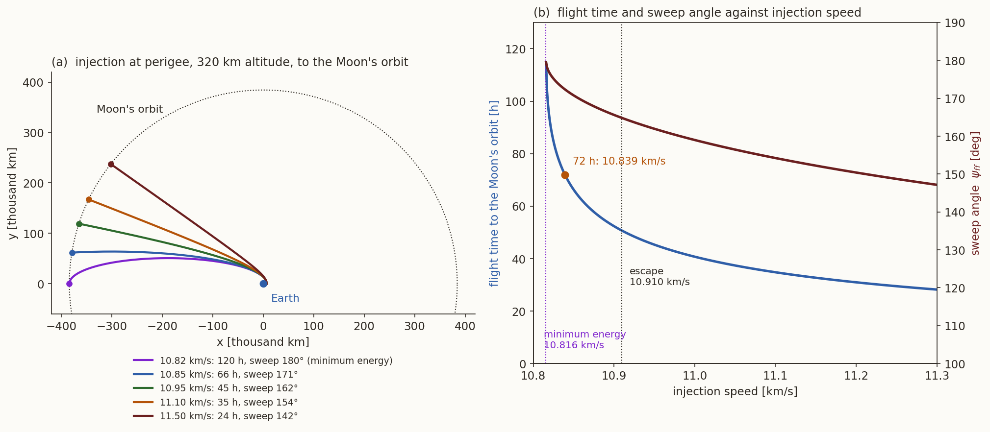
Two things should strike you. First, the flight time is very sensitive near the minimum speed and not at all sensitive away from it: \(23.4\) m/s above the minimum, \(0.2\%\) of the injection speed, shortens the flight from \(119.5\) h to \(72\) h, a saving of \(47.5\) h; to get below about \(41\) h one needs another \(160\) m/s. Second, the faster flights are almost radial (\(\gamma_D\approx85^\circ\) at arrival): there is a near straight line from the Earth to the Moon. For a crewed mission the life-support mass grows with the flight time, so the extra speed pays for itself up to a point; Bate quotes about \(72\) hours for the Apollo landing missions. The speed that gives exactly \(72\) h in the present model is \(10.839\) km/s.
2.3 The minimum-energy flight
If the injection speed is lowered, the apogee of the orbit falls, and the lowest speed that still reaches the Moon’s orbit is the one whose apogee is exactly at \(r=D\). For a perigee injection the perigee and apogee distances are \(r_0\) and \(D\), so
\[ a_0=\frac{r_0+D}{2},\qquad e_0=\frac{D-r_0}{D+r_0},\qquad v_{min}=\sqrt{\frac{2\mu_\oplus D}{r_0\,(r_0+D)}},\qquad t_{max}=\pi\sqrt{\frac{a_0^3}{\mu_\oplus}} . \tag{4}\]
(\(v_{min}\) follows from the vis-viva equation at perigee, \(v^2=\mu(2/r_0-1/a_0)\).) With \(r_0=6698.137\) km: \(a_0=195\,549\) km, \(e_0=0.9657\), \(v_{min}=10.816\) km/s, and the flight takes \(t_{max}=119.5\) h \(=7172\) min. This is the longest flight that reaches the Moon; anything slower never gets there. The sweep angle is exactly \(180^\circ\) and the arrival is at apogee, where the velocity is purely horizontal, of size \(h_0/D=v_{min}r_0/D=0.1885\) km/s, in the same direction as the Moon’s own motion. The Moon moves at \(1.0245\) km/s, so it comes up to the probe from behind at the closing speed \(0.836\) km/s, and the impact is on the Moon’s leading hemisphere. (Bate: \(0.188\) km/s.)
Compute \(v_{min}\), \(e_0\) and \(t_{max}\) for a perigee injection at \(r_0=6698.137\) km.
What you should find
\(2\mu_\oplus D=3.0644\times10^{11}\); \(r_0(r_0+D)=6698.137\times391\,098.1=2.6196\times10^9\); the ratio is \(116.98\) and \(v_{min}=10.816\) km/s. \(e_0=(384\,400-6698.137)/(391\,098.1)=0.9657\). \(a_0=195\,549\) km, \(\sqrt{a_0^3/\mu_\oplus}=136\,970\) s, times \(\pi\) is \(430\,290\) s \(=119.5\) h.Why does the flight time fall so quickly at the beginning, \(23\) m/s buying \(47\) hours?
Answer
At the minimum speed the vehicle reaches the Moon’s orbit at apogee, where it is moving almost not at all (\(0.19\) km/s) and spends a very long time. A little more energy moves the apogee beyond the Moon’s orbit, and the vehicle crosses the orbit at a point before apogee, still moving at \(0.4\) to \(0.9\) km/s, not \(0.19\). The time spent near apogee, where the vehicle crawls, is cut off. Mathematically \(dt/dv_0\to-\infty\) at \(v_{min}\) because of the square-root behaviour of the time near the turning point. (Bate’s Fig. 7.3-1.)2.4 Where does the vehicle meet the Moon? The effect of injection errors
If the engine does not deliver the planned \((r_0,v_0,\gamma_0)\), the vehicle crosses the Moon’s orbit at a different place and a different time, so it meets the Moon’s orbit at some other point. To be hit by the Moon the vehicle has to be at the Moon’s position at the time of crossing, so what matters is the difference of two angles: where the vehicle crosses (the sweep angle from the injection point) and where the Moon is (its angle at the planned injection moment plus the angle it travels in the flight time). With the Moon at \(\gamma_{dep}\) ahead of the injection point at the instant of injection (the phase angle at departure), the vehicle arrives at the angle \(\psi_{ff}\) while the Moon is at \(\gamma_{dep}+n_{\rm Moon}t_{ff}\) (we take direct motion, both going the same way round the Earth). The miss along the Moon’s orbit is
\[ \text{miss}=D\bigl(\psi_{ff}-n_{\rm Moon}\,t_{ff}-\gamma_{dep}\bigr),\qquad \Delta(\text{miss})=D\,\Delta\bigl(\psi_{ff}-n_{\rm Moon}\,t_{ff}\bigr) . \tag{5}\]
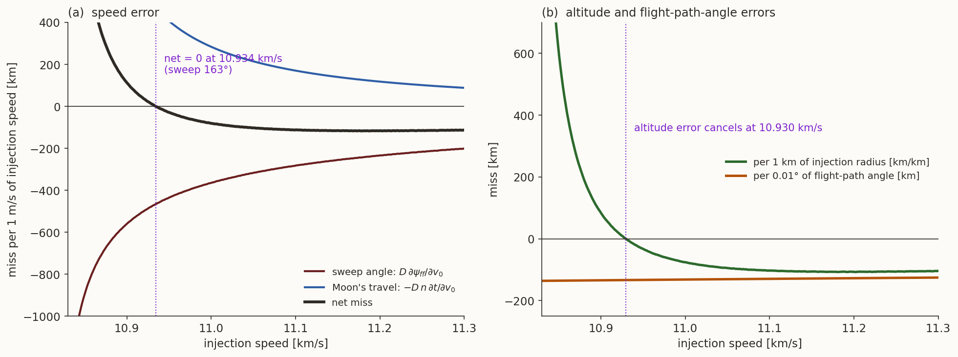
The two terms in the bracket have the same sign of change for most errors, and so they cancel. If the injection speed is too high, the vehicle sweeps a smaller angle (it is more nearly radial) and arrives earlier, so the Moon, which has had less time, is also behind the planned position. Both \(\Delta\psi_{ff}<0\) and \(-n_{\rm Moon}\Delta t_{ff}>0\) for a speed that is too high: the miss is the difference of the two (Figure 2).
The result:
- Speed and altitude errors nearly cancel at an injection speed of about \(10.93\) km/s, which gives a sweep angle of \(163^\circ\) and a flight time of \(47\) h. At \(11.0\) km/s the net miss is \(-81\) km per m/s of speed error (made up of \(-365\) from the sweep and \(+284\) from the Moon’s motion) and \(-76\) km per km of altitude error. (Bate says that the two cancel at “about \(11.0\) km/s, sweep about \(160^\circ\)”; the exact value in this model is \(10.93\) km/s and \(163^\circ\).) This is why lunar flights are flown at about this speed: the miss is then insensitive to the two errors that are hardest to control.
- A flight-path angle error does not cancel. One degree in \(\gamma_0\) moves the arrival point by \(13\,200\) km along the Moon’s orbit, at any speed in the range. (Bate prints “about \(1300\) km for \(1^\circ\)”; direct integration of the equations of motion gives \(1318\) km for \(0.1^\circ\) and \(13\,180\) km for \(1^\circ\), so Bate’s number appears to belong to a tenth of a degree.) The reason is that the injection is near the perigee of a very eccentric ellipse: for \(e\to1\) the relation \(\tan\gamma=e\sin f/(1+e\cos f)\) becomes \(\tan\gamma=\tan(f/2)\), so \(f_0\approx2\gamma_0\) and the sweep angle \(\psi_{ff}=f_D-f_0\) changes by about \(-2\Delta\gamma_0\): \(2^\circ\) per degree, which is \(13\,400\) km at the Moon’s distance. The direction of the burn must be accurate to a few hundredths of a degree.
Two caveats. These numbers neglect the Moon’s gravity, which pulls a vehicle that passes it towards it and reduces the miss (Bate). And a real mission does not rely on the injection being exact; it carries a trajectory correction manoeuvre a day or so into the flight, when the errors can be measured and removed at a small cost in speed.
3 The patched-conic approximation
To predict where the vehicle goes near the Moon we have to include the Moon’s attraction. The patched-conic idea (patched-conics note): inside the Moon’s sphere of influence of radius \(r_{\rm SOI}\) (Table 1) the vehicle is attracted by the Moon alone, outside by the Earth alone, and the two conics are joined at the sphere’s surface by matching the position and (the Moon’s motion being allowed for) the velocity. The derivation of \(r_{\rm SOI}\), the argument for the velocity matching and a complete example are in that note (sphere of influence, Example 2). Here we give the procedure in Bate’s order, derive the equations that note takes for granted, and work Bate’s own example.
3.1 The independent variables
The geocentric leg is fixed by the injection conditions \((r_0,v_0,\gamma_0)\), and the point where it crosses the sphere of influence must be found. Bate’s trick is to choose that point rather than to find it: take as the fourth independent variable the angle
\[ \lambda_1=\text{the angle at the Moon between the line to the Earth and the line to the patch point} \]
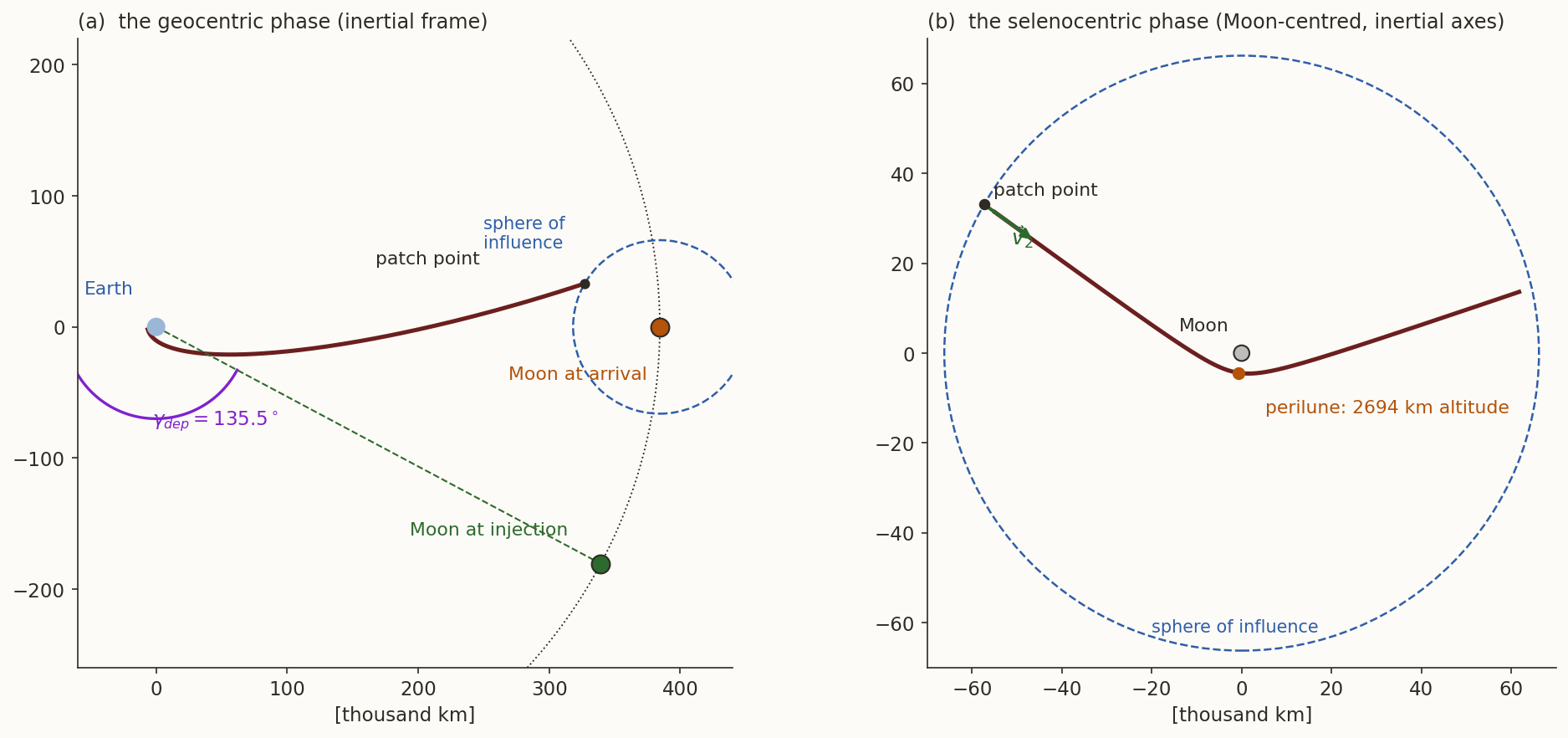
(Figure 3 (a); the patch point is on the side of the Moon’s motion, so that the vehicle meets it in front). Given \((r_0,v_0,\gamma_0,\lambda_1)\) everything else follows in closed form, whereas choosing \(\gamma_0\) and \(v_0\) and finding where the conic crosses the sphere needs a trial and error with a flight time in the loop. The price is that the answer, a perilune, is only known at the end; then \((v_0,\gamma_0,\lambda_1)\) are adjusted by trial until the perilune is right. The flight is assumed to be direct, arriving before the apogee of the geocentric conic, so that \(0<\gamma_1<90^\circ\).
3.2 The geocentric leg
The conic: \(\varepsilon_0\), \(h_0\), \(p_0\), \(e_0\) from Equation 1.
The patch point. In the triangle Earth–Moon–patch point two sides are known, \(D\) and \(r_{\rm SOI}\), and the angle between them, \(\lambda_1\). The cosine rule gives the geocentric distance of the patch point, and the sine rule the angle \(\eta_1\) at the Earth between the Moon and the patch point:
\[ r_1=\sqrt{D^2+r_{\rm SOI}^2-2Dr_{\rm SOI}\cos\lambda_1},\qquad \sin\eta_1=\frac{r_{\rm SOI}}{r_1}\sin\lambda_1 . \tag{6}\]
The state at the patch point. Energy and angular momentum are conserved: \(v_1=\sqrt{2(\varepsilon_0+\mu_\oplus/r_1)}\) and \(\cos\gamma_1=h_0/(r_1v_1)\). If \(\varepsilon_0+\mu_\oplus/r_1<0\) the vehicle does not reach the sphere of influence; that is the failure mode of this procedure, and it means that \(v_0\) was too small.
The time of flight. The true anomalies at injection and at the patch point are \(\cos f=(p_0/r-1)/e_0\) at \(r_0\) and \(r_1\) (for \(\gamma_0\ge0\), \(f_0\ge0\), and \(f_1\in(0,\pi)\) on the outbound leg), the eccentric anomalies follow from \(\tan(E/2)=\sqrt{(1-e_0)/(1+e_0)}\tan(f/2)\), and \[ t_1=\sqrt{\frac{a_0^3}{\mu_\oplus}}\Bigl[(E_1-e_0\sin E_1)-(E_0-e_0\sin E_0)\Bigr] . \tag{7}\]
The phase angle at departure. The vehicle sweeps the geocentric angle \(f_1-f_0\) between injection and the patch point. At the patch point it is at the angle \(\eta_1\) ahead of the Moon’s centre (as seen from the Earth). So at that moment the Moon is at \(f_1-f_0-\eta_1\) from the injection point. In the flight time \(t_1\) the Moon has moved \(n_{\rm Moon}t_1\). Hence at injection the Moon must be ahead of the injection point by
\[ \boxed{\gamma_{dep}=f_1-f_0-\eta_1-n_{\rm Moon}\,t_1}\ . \tag{8}\]
This is Bate’s (7.4-16). It fixes the launch time: injection must happen when the Moon is \(\gamma_{dep}\) ahead of the injection point.
3.3 The velocity relative to the Moon
At the patch point the vehicle’s geocentric velocity \(\mathbf v_1\) is changed to the velocity relative to the Moon, \(\mathbf v_2=\mathbf v_1-\mathbf v_{\rm Moon}\), where \(\mathbf v_{\rm Moon}\) (of length \(v_{\rm Moon}\), perpendicular to the Earth–Moon line) is the velocity of the Moon at that moment, and the position relative to the Moon is \(\boldsymbol\rho\), of length \(r_{\rm SOI}\) (the Moon-to-patch-point vector). The angle between \(\mathbf v_1\) and \(\mathbf v_{\rm Moon}\) is \(\gamma_1-\eta_1\) (patched-conics note, Step 5: the Moon’s velocity is turned by \(\eta_1\) from the local horizontal at the patch point, the vehicle’s by \(\gamma_1\)). The cosine rule for the third side of the velocity triangle gives
\[ v_2=\sqrt{v_1^2+v_{\rm Moon}^2-2\,v_1v_{\rm Moon}\cos(\gamma_1-\eta_1)} . \tag{9}\]
What we need next is how the velocity \(\mathbf v_2\) is directed with respect to the line to the Moon’s centre. Define the aiming angle \(\zeta_2\) as the angle between \(\mathbf v_2\) and the direction from the patch point to the Moon’s centre (Bate’s \(\epsilon_2\); it is zero if the vehicle heads for the centre of the Moon). The component of \(\mathbf v_2\) perpendicular to \(\boldsymbol\rho\) is \(v_2\sin\zeta_2\), and the angular momentum about the Moon is \(h_2=r_{\rm SOI}\,v_2\sin\zeta_2\). Because \(\mathbf v_2=\mathbf v_1-\mathbf v_{\rm Moon}\), that component is the difference of the same components of \(\mathbf v_1\) and \(\mathbf v_{\rm Moon}\). The Moon’s velocity is perpendicular to the Earth–Moon line, and \(\boldsymbol\rho\) makes the angle \(\lambda_1\) with that line, so \(\mathbf v_{\rm Moon}\) makes the angle \(\lambda_1\) with the direction perpendicular to \(\boldsymbol\rho\) and has the perpendicular component \(v_{\rm Moon}\cos\lambda_1\) (check: for \(\lambda_1=0\), \(\boldsymbol\rho\) lies along the line and the whole of \(\mathbf v_{\rm Moon}\) is perpendicular to it). The vehicle’s velocity \(\mathbf v_1\) is turned from \(\mathbf v_{\rm Moon}\) by \(\gamma_1-\eta_1\) (above), towards the outward radial direction, so it makes the angle \(\lambda_1-(\gamma_1-\eta_1)=\lambda_1+\eta_1-\gamma_1\) with the same perpendicular, and its perpendicular component is \(v_1\cos(\lambda_1+\eta_1-\gamma_1)\). Taking the difference,
\[ h_2=r_{\rm SOI}\,v_2\sin\zeta_2=r_{\rm SOI}\Bigl[v_{\rm Moon}\cos\lambda_1-v_1\cos(\lambda_1+\eta_1-\gamma_1)\Bigr] . \tag{10}\]
This is Bate’s (7.4-20) with \(h_2\) in place of \(\sin\epsilon_2\). The script confirms it against a construction with explicit vectors in the Earth–Moon plane, which also supplies the sign: \(h_2>0\) means that the vehicle goes round the Moon in the same sense as the Moon goes round the Earth (direct), \(h_2<0\) opposite (retrograde). For a dead-centre hit, \(h_2=0\).
3.4 The selenocentric leg
Inside the sphere the Moon alone attracts. The vehicle arrives with the speed \(v_2\) at the distance \(r_{\rm SOI}\) with the angular momentum \(h_2\), and the conic is fixed:
\[ \varepsilon_2=\frac{v_2^2}{2}-\frac{\mu_{\rm Moon}}{r_{\rm SOI}},\qquad p_2=\frac{h_2^2}{\mu_{\rm Moon}},\qquad e_2=\sqrt{1+\frac{2\varepsilon_2h_2^2}{\mu_{\rm Moon}^2}},\qquad r_p=\frac{p_2}{1+e_2},\qquad v_p=\sqrt{2\Bigl(\varepsilon_2+\frac{\mu_{\rm Moon}}{r_p}\Bigr)} . \tag{11}\]
The energy is positive when \(v_2>\sqrt{2\mu_{\rm Moon}/r_{\rm SOI}}=0.385\) km/s, the escape speed from the Moon at the boundary of its sphere. A vehicle coming from the Earth arrives at about the Moon’s own speed or less relative to the Moon, around \(1\) km/s (\(1.2\) km/s in the example), far above that, so the selenocentric conic is a hyperbola: a vehicle that arrives from the Earth is not captured by the Moon unless it brakes. (Bate asks why \(\varepsilon_2>0\).) The perilune radius \(r_p\) is the main output, and three missions are possible:
- Impact: \(r_p<R_{\rm Moon}=1737.4\) km; the impact speed follows from the energy, \(v=\sqrt{2(\varepsilon_2+\mu_{\rm Moon}/R_{\rm Moon})}\).
- Lunar orbit: brake at perilune to a circular orbit with \(\Delta v=v_p-\sqrt{\mu_{\rm Moon}/r_p}\).
- Circumlunar flight: coast through perilune and leave the sphere again (the return trajectory; see the limits below).
3.5 Bate’s example
Example 1 (injection to the Moon). The vehicle is injected at perigee, \(r_0=6698.137\) km, with \(v_0=10.846\) km/s (\(1.372\) circular speeds at the Earth’s surface), \(\gamma_0=0\), and crosses the sphere of influence at \(\lambda_1=30^\circ\). Find the phase angle at departure and the closest approach.
Solution.
Geocentric orbit. \(\varepsilon_0=v_0^2/2-\mu_\oplus/r_0=-0.6913\) km\(^2\)/s\(^2\), \(h_0=r_0v_0=72\,648\) km\(^2\)/s, \(p_0=13\,241\) km, \(a_0=288\,301\) km, \(e_0=0.9768\).
The patch point. \(r_1=\sqrt{384\,400^2+66\,183^2-2(384\,400)(66\,183)\cos30^\circ}=328\,754\) km, \(\sin\eta_1=(66\,183/328\,754)\sin30^\circ\), \(\eta_1=5.777^\circ\).
The state there. \(v_1=\sqrt{2(-0.6913+398\,600.4/328\,754)}=1.0209\) km/s and \(\cos\gamma_1=72\,648/(328\,754\times1.0209)\), \(\gamma_1=77.50^\circ\) (the vehicle is still climbing steeply). The true anomaly there is \(f_1=169.28^\circ\), and Equation 7 gives \(t_1=50.97\) h.
The phase angle. With \(f_0=0\) and \(n_{\rm Moon}t_1=2.6653\times10^{-6}\times183\,477=0.4890\) rad \(=28.02^\circ\): \(\gamma_{dep}=169.28^\circ-5.78^\circ-28.02^\circ=135.48^\circ\) (\(135.49^\circ\) with the unrounded values). The Moon must be \(135.5^\circ\) ahead of the vehicle at injection.
Velocity relative to the Moon. Equation 9: \(v_2=\sqrt{1.0209^2+1.0245^2-2(1.0209)(1.0245)\cos(77.50^\circ-5.78^\circ)}=1.1983\) km/s. Equation 10: \(h_2=66\,183\,[1.0245\cos30^\circ-1.0209\cos(30^\circ+5.78^\circ-77.50^\circ)]=66\,183\,(0.8873-0.7620)=8291\) km\(^2\)/s, so \(\sin\zeta_2=8291/(66\,183\times1.1983)\), \(\zeta_2=6.00^\circ\) (positive: direct about the Moon).
The hyperbola. \(\varepsilon_2=1.1983^2/2-4902.8/66\,183=0.6439\) km\(^2\)/s\(^2\) (\(v_\infty=\sqrt{2\varepsilon_2}=1.1348\) km/s), \(p_2=8291^2/4902.8=14\,020\) km, \(e_2=\sqrt{1+2(0.6439)(8291)^2/4902.8^2}=2.1639\), and
\[ r_p=\frac{14\,020}{1+2.1639}=4431\ \text{km}, \]
an altitude of \(2694\) km above the Moon’s surface. The speed at perilune is \(v_p=1.871\) km/s, and the circular speed at that radius \(1.052\) km/s, so capture into a circular lunar orbit would need a braking burn of \(0.819\) km/s. The vehicle does not hit the Moon.
Comparison with the book. Bate’s printed values include \(v_2=1.198\) km/s and \(\varepsilon_2=0.6437\) km\(^2\)/s\(^2\), which agree with ours. His other numbers are a few percent off ours (\(t_1=50.2\) h, \(\gamma_{dep}=135.9^\circ\), \(e_2=2.078\)): he works to three or four digits in canonical units, and in this problem \(\varepsilon_0\) is a small difference of two large numbers (\(v_0^2/2=58.8\), \(\mu_\oplus/r_0=59.5\), difference \(-0.69\)), so rounding it to \(-0.011\) canonical units (instead of \(-0.0111\)) changes \(v_1\) by \(1\%\), and the rest follows. The same rounding is a warning about how well the whole procedure is conditioned.
3.6 How sensitive is it, and how good?
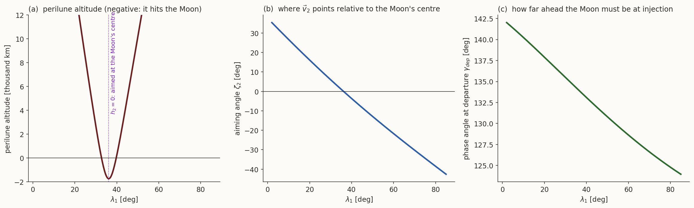
The perilune is the difference of large effects, and the vehicle passes the Moon at about its own speed relative to it, so it is very sensitive to the choice of \(\lambda_1\). Figure 4 (a) shows the perilune altitude for the injection of Example 1 against \(\lambda_1\): it falls by about \(1080\) km per degree of \(\lambda_1\) at \(30^\circ\) and reaches the Moon’s surface, so the vehicle hits it, for \(32.7^\circ<\lambda_1<39.7^\circ\), a window of only \(7^\circ\) around the value \(\lambda_1=36.16^\circ\) for which \(h_2=0\) and the vehicle is aimed at the Moon’s centre. The sign of \(h_2\) changes there: for smaller \(\lambda_1\) the vehicle passes the Moon on the near side and goes round it in the direct sense, for larger in the retrograde sense. The phase angle at departure falls by about \(0.24^\circ\) per degree of \(\lambda_1\) (panel c), so that the time at which the engine must fire is also adjustable.
How good is the patched conic? To find out we repeat the flight with the equation of motion that includes both attractions throughout. In the Earth-centred frame, with the Moon on its circle and starting at the phase angle \(\gamma_{dep}\) of Equation 8,
\[ \ddot{\mathbf r}=-\mu_\oplus\frac{\mathbf r}{r^3}+\mu_{\rm Moon}\Bigl[\frac{\mathbf r_{\rm Moon}-\mathbf r}{|\mathbf r_{\rm Moon}-\mathbf r|^3}-\frac{\mathbf r_{\rm Moon}}{r_{\rm Moon}^3}\Bigr], \tag{12}\]
where the last term is the acceleration of the Earth towards the Moon, which has to be subtracted because the frame is attached to the Earth. Integrating it from the same injection, the closest approach to the Moon is at \(3192\) km altitude at \(64.66\) h, against \(2694\) km at \(65.3\) h (\(50.97\) h to the sphere, \(14.4\) h more along the hyperbola) for the patched conic. The error is \(500\) km in perilune (\(0.2\%\) of the Earth–Moon distance, but \(19\%\) of the perilune altitude) and \(0.7\) h in time. The same code applied to the injection of the patched-conics note (its Example 2) reproduces what is printed there: \(1030\) km at \(87.0\) h, where the patched conic says \(1627\) km, an error of \(600\) km. Bate remarks that the patched conic is good for the outbound \(\Delta v\), but not for the return trajectory, where the error at the sphere of influence is amplified, and not for the orientation of the lunar orbit. For the Moon it is a good first guess for a numerical search (Bate’s exercise 7.11), never the answer.
In Figure 4 (a) the vehicle hits the Moon only for a \(7^\circ\) window of \(\lambda_1\), and the perilune altitude is a smooth curve, but the patched-conic error is \(500\) km. How wide in \(\lambda_1\) is the error, in other words by how much would \(\lambda_1\) have to be shifted for the patched conic to reproduce the true perilune?
Answer
By \(500/1080\approx0.5^\circ\). The patched-conic answer is wrong by half a degree of \(\lambda_1\), which is \(0.5^\circ\times66\,183\) km \(\times\pi/180\approx580\) km along the sphere of influence’s surface. A lunar mission is therefore planned with the patched conic and then corrected by numerical integration: the patched conic is used to find an injection that is within a fraction of a degree of the right one.What the check is. The restricted integration of Equation 12 is in lunar-verify.py, and is itself checked on the one case that the patched-conics note reports (closest approach of \(1030\) km at \(87.0\) h). The formulas of this section (Equation 6 to Equation 11) are checked against that note’s Example 2: \(r_1\), \(\eta_1\), \(v_1\), \(\gamma_1\), \(t_1\), \(v_2\), \(h_2\), \(e_2\), \(r_p\) and \(\gamma_{dep}\) all agree.
4 Launching from a site whose latitude is not the Moon’s
So far the vehicle’s plane was the Moon’s plane. It is not a matter of choice: a launch from latitude \(\delta_0\) can put the vehicle into a parking orbit only of inclination \(i\ge|\delta_0|\), and the plane of the transfer is fixed by the plane of the launch and the way the vehicle gets to injection. The Moon’s orbit has an inclination to the equator between \(18.3^\circ\) and \(28.6^\circ\), with the \(18.6\)-year period of Section 1. A launch site at \(28.5^\circ\)N (the Kennedy Space Center) can reach the Moon’s plane for the whole month only when that plane has its largest inclination, which last happened in 1969; Bate says it would happen again in 1978, but the inclination is smallest then, and the maxima are \(18.6\) years apart: after 1969 the next is about 1987, then 2006 and 2024–25. At every other time the transfer plane is not the Moon’s plane, and the vehicle crosses the Moon’s orbit at one point of it, where the Moon must be.
4.1 The sweep angle and the declination at intercept
The transfer from launch to intercept is a great circle on the celestial sphere (a plane through the Earth’s centre). Measured along it, the total geocentric angle from the launch point to the intercept point is the total sweep angle
\[ \psi_t=\psi_c+\psi_{ff} , \tag{13}\]
where \(\psi_{ff}\) is the free-flight sweep of Section 2 (a function of the injection conditions, Table 2) and \(\psi_c\) is the angle swept between launch and injection: the burning arc for a direct ascent, or the burning arc plus the coast in a parking orbit. We can choose \(\psi_c\) freely; the injection conditions fix \(\psi_{ff}\).
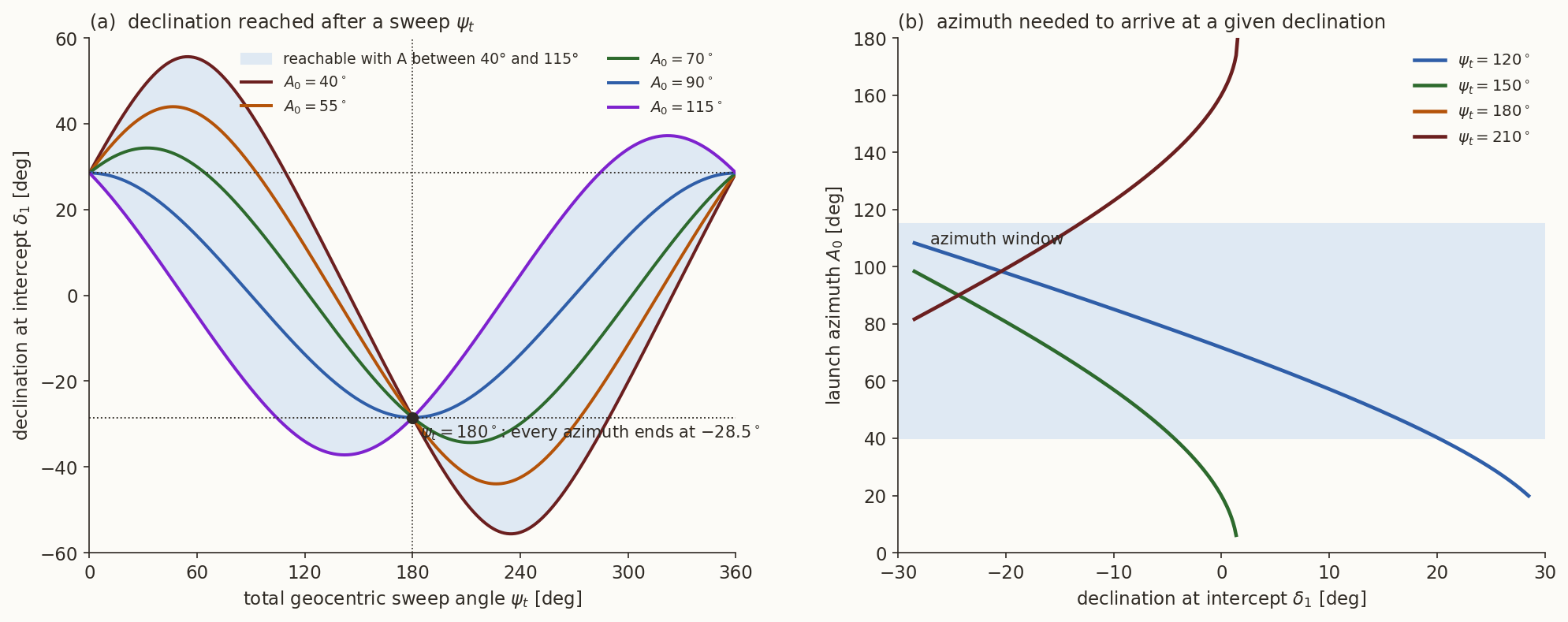
Now two points on the celestial sphere: the launch point (declination \(\delta_0\) equal to the site latitude, right ascension \(\alpha_0\) equal to the local sidereal time) and the intercept point (declination \(\delta_1\), right ascension \(\alpha_1\)), at the angular distance \(\psi_t\) along a great circle that leaves the launch point at the azimuth \(A_0\) (from north, clockwise). In the spherical triangle with the pole \(N\), the launch point and the intercept point, the sides are \(90^\circ-\delta_0\), \(90^\circ-\delta_1\) and \(\psi_t\), and the angle at the launch point is \(A_0\) (the angle at the pole is \(\alpha_1-\alpha_0\) in magnitude). The law of cosines for the side \(90^\circ-\delta_1\) gives
\[ \boxed{\sin\delta_1=\sin\delta_0\cos\psi_t+\cos\delta_0\sin\psi_t\cos A_0} , \tag{14}\]
which can also be seen with vectors: moving from the launch point \(\hat{\mathbf P}_0\) a distance \(\psi_t\) along the great circle that leaves in the direction \(\hat{\mathbf t}=\cos A_0\hat{\mathbf N}+\sin A_0\hat{\mathbf E}\) gives \(\hat{\mathbf P}_1=\cos\psi_t\hat{\mathbf P}_0+\sin\psi_t\hat{\mathbf t}\), and the \(z\) component of this is \(\sin\delta_1\), because \(\hat{\mathbf P}_0\) has the \(z\) component \(\sin\delta_0\) and the north unit vector \(\cos\delta_0\), the east one \(0\). Solving for the azimuth, and using the law of cosines for the side \(\psi_t\) to find the difference of right ascension,
\[ \cos A_0=\frac{\sin\delta_1-\sin\delta_0\cos\psi_t}{\cos\delta_0\sin\psi_t},\qquad \cos\Delta\alpha=\frac{\cos\psi_t-\sin\delta_0\sin\delta_1}{\cos\delta_0\cos\delta_1} . \tag{15}\]
(Bate’s (7.5-3) and (7.5-4); the script checks Equation 14 and Equation 15 against the explicit vector construction in 200 random cases.) The \(\Delta\alpha\) of Equation 15 is the angle at the pole, so it lies between \(0\) and \(180^\circ\). The eastward difference in right ascension, which is what a launch time depends on, equals it for \(\psi_t\le180^\circ\) and equals \(360^\circ-\Delta\alpha\) for \(\psi_t>180^\circ\) (when the path is eastward, \(0<A_0<180^\circ\)), because then the path has gone more than half-way round.
What Equation 14 says.
- For a given sweep \(\psi_t\) and launch site, the declination at intercept lies between the values for a due-north launch (\(A_0=0\): \(\sin\delta_1=\sin(\delta_0+\psi_t)\)) and a due-south launch (\(A_0=180^\circ\): \(\sin\delta_1=\sin(\delta_0-\psi_t)\)). For \(\delta_0=28.5^\circ\) and \(\psi_t=150^\circ\) that is \(\delta_1\in[-58.5^\circ,\,1.5^\circ]\).
- The intercept declination and the launch azimuth are not independent: once \(\psi_t\) is chosen, one fixes the other (Equation 15). The range-safety rules of the launch site limit the azimuth: Bate uses \(40^\circ\le A_0\le115^\circ\) for the Eastern Test Range. With it, \(\psi_t=150^\circ\) gives \(\delta_1\in[-36.8^\circ,\,-4.4^\circ]\) (Figure 5 (a)), and since the Moon’s declination is limited to \(\pm28.5^\circ\) (1969), the usable part is \([-28.5^\circ,-4.4^\circ]\): the Moon must be south of the equator at intercept, in the south half of its monthly swing.
- A sweep of exactly \(180^\circ\) gives \(\sin\delta_1=-\sin\delta_0\) for every azimuth: all the great circles from a point meet at the antipode. So \(\psi_t=180^\circ\) can be flown only to the Moon at its extreme southern declination \(-\delta_0\); the azimuth is then free.
- Since the least injection speed gives \(\psi_{ff}\) near \(180^\circ\) (Table 2), a direct ascent (\(\psi_c\) small) has \(\psi_t\) near \(\psi_{ff}\), and can reach the Moon only when its declination is in a narrow range near \(-\delta_0\). Bate: free-flight sweeps of less than about \(120^\circ\) need very high injection speeds, so a cheap direct launch can intercept the Moon only near its maximum southern declination. If a coast arc \(\psi_c\) is added that makes \(\psi_t>180^\circ\), the vehicle can intercept the Moon at any declination: this is why real missions go through a parking orbit.
Why does the sweep of exactly \(180^\circ\) make the launch azimuth irrelevant?
Answer
Every great circle through a point on a sphere also passes through the antipodal point, after exactly \(180^\circ\). The antipode of the launch point has the declination \(-\delta_0\), whatever the azimuth of the great circle through it. The same fact is why a missile flight of \(180^\circ\) lands on the antipode whatever the azimuth (ballistic note, where \(\Delta C=\Delta A\sin\psi\) vanishes at \(\psi=180^\circ\)).4.2 Choosing the date and the launch time
Having found how the three angles are tied, the procedure for finding a launch time is Bate’s. The Moon’s right ascension and declination are tabulated for each hour in an ephemeris; the sidereal time of the launch site depends on the time of day. The steps:
- Choose the injection conditions \((r_0,v_0,\gamma_0)\) and the coast \(\psi_c\). They give \(\psi_{ff}\) and \(t_{ff}\) (Section 2.1), hence \(\psi_t\) (Equation 13) and the total time from launch to intercept \(t_t=t_{ff}+t_c\), where \(t_c\) is the time of the burn and the coast.
- Choose the declination \(\delta_1\) at intercept, subject to the lighting conditions on the Moon (the phase) and to the azimuth window; then Equation 15 gives the launch azimuth \(A_0\), which must be inside the window.
- Search the ephemeris for a time \(t_1\) at which the Moon’s declination is \(\delta_1\) (and whose phase is acceptable), and take the Moon’s right ascension \(\alpha_1\) at that time.
- The required right ascension of the launch point is the Moon’s minus the eastward difference of Equation 15: \(\alpha_0=\alpha_1-\Delta\alpha_E\). The right ascension of the launch site equals the local sidereal time, \(\alpha_0=\theta_G+\lambda_E\) (\(\theta_G\) the Greenwich sidereal angle, \(\lambda_E\) the east longitude of the site; time note).
- The launch time is \(t_0=t_1-t_t\) (Equation 13, the total time of flight). It is the time at which the sidereal time of the site reaches the \(\alpha_0\) of step 4.
It would be a coincidence if the sidereal time at \(t_0\) were the required one. The site’s right ascension advances \(360.99^\circ\) per day, but the Moon’s changes by only \(13^\circ\) per day, so moving the intercept time \(t_1\) by up to a day (at the price of a change of the Moon’s declination, typically a few degrees per day, so that the azimuth must be recomputed) brings the two into agreement. In practice this means that for each lunar month there is one launch opportunity per sidereal day for a given declination, and the daily launch windows move through the month.
Example 2 (the geometry of a launch). Take the injection of \(10.9345\) km/s at perigee (\(320\) km altitude): \(\psi_{ff}=162.99^\circ\) and \(t_{ff}=47.13\) h, the speed at which speed and altitude errors cancel (Section 2.4). Add a burn-plus-coast arc \(\psi_c=27^\circ\) (in a \(320\) km parking orbit, whose angular rate is \(\sqrt{\mu_\oplus/r_0^3}=1.1465\times10^{-3}\) rad/s, that takes \(6.8\) min). The total sweep is \(\psi_t=190^\circ\) and \(t_t=47.25\) h. The launch site is at \(\delta_0=28.5^\circ\) and the Moon is at \(\delta_1=-25^\circ\) at intercept.
Azimuth. Equation 15: \(\cos A_0=\dfrac{\sin(-25^\circ)-\sin28.5^\circ\cos190^\circ}{\cos28.5^\circ\sin190^\circ}=\dfrac{-0.4226+0.4699}{-0.1526}=-0.310\), so \(A_0=108.05^\circ\): inside the window \(40^\circ\) to \(115^\circ\).
Right ascension. \(\cos\Delta\alpha=\dfrac{\cos190^\circ-\sin28.5^\circ\sin(-25^\circ)}{\cos28.5^\circ\cos(-25^\circ)}=\dfrac{-0.9848+0.2017}{0.7965}=-0.9832\), \(\Delta\alpha=169.50^\circ\) at the pole. Because \(\psi_t>180^\circ\), the eastward difference is \(360^\circ-169.50^\circ=190.50^\circ\) (the script confirms it by following the great circle). So the launch site must have the right ascension \(\alpha_0=\alpha_1-190.5^\circ=\alpha_1+169.5^\circ\) at the launch time, which is \(47.25\) h before the intercept.
A site closer to the equator is more restricted, not less. For a launch site at \(13.7^\circ\)N (Sriharikota) and the same \(\psi_t=190^\circ\), Equation 14 bounds the declination at intercept to \(\sin\delta_1\in\sin13.7^\circ\cos190^\circ\pm\cos13.7^\circ\sin190^\circ\), that is \(\delta_1\in[-23.7^\circ,\,-3.7^\circ]\) for any azimuth at all; a Moon at \(-25^\circ\) cannot be reached with this sweep, whatever the azimuth. The remedy is the one that Bate points out: a different coast \(\psi_c\). A long phase in Earth orbit before the injection burn, as in the Chandrayaan missions, which raise the orbit in several perigee burns before the translunar injection (see the Indian missions problems), has this geometric benefit among others: the coast arc \(\psi_c\) can be chosen, so the time of the injection burn can be chosen to suit the Moon’s position, whatever the launch site’s latitude.
Summary
In one paragraph. The Earth–Moon system has a barycentre inside the Earth, the Moon on a nearly circular orbit of radius \(384\,400\) km with speed \(1.02\) km/s, and a sphere of influence of \(66\,183\) km. Ignoring the Moon’s gravity, a perigee injection at \(320\) km altitude reaches the Moon’s orbit if \(v_0\ge10.816\) km/s (\(119.5\) h, sweep \(180^\circ\)); a speed \(23\) m/s higher gives \(72\) h and \(10.934\) km/s gives \(47\) h, where speed and altitude errors cancel in the miss \(D\Delta(\psi_{ff}-n_{\rm Moon}t_{ff})\) but a flight-path angle error of one degree still gives \(13\,000\) km. The patched conic joins a geocentric conic to a selenocentric one at the angle \(\lambda_1\) on the sphere of influence: \(r_1\), \(\eta_1\), \(v_1\), \(\gamma_1\), \(t_1\), the phase angle at departure \(\gamma_{dep}=f_1-f_0-\eta_1-n_{\rm Moon}t_1\), then \(v_2\), \(h_2=r_{\rm SOI}[v_{\rm Moon}\cos\lambda_1-v_1\cos(\lambda_1+\eta_1-\gamma_1)]\) and the hyperbola of perilune \(r_p\); it is sensitive (\(1080\) km per degree of \(\lambda_1\)) and about \(500\) km off in perilune in the example. A launch from latitude \(\delta_0\) with a total sweep \(\psi_t\) and azimuth \(A_0\) reaches the declination given by \(\sin\delta_1=\sin\delta_0\cos\psi_t+\cos\delta_0\sin\psi_t\cos A_0\), which with range-safety limits on the azimuth and a direct ascent allows the Moon only in a narrow part of the month; a coast arc making \(\psi_t>180^\circ\) removes the restriction.
The numbers of this note are checked by lunar-verify.py, using the helper module _lunar.py; the figure scripts are fig-lun-flight.py (which draws both Figure 1 and Figure 2), fig-lun-patch.py (Figure 3 and Figure 4) and fig-lun-noncoplanar.py.
What we left out. (i) Precise trajectories: numerical integration with the Earth’s oblateness, the Sun and a lunar ephemeris, in which the Moon’s orbit has its true eccentricity and plane. (ii) Return trajectories and free return: a trajectory that swings round the Moon and returns to the Earth with no further burn, the Apollo 13 safety net; the patched conic is not accurate enough to design it (Bate’s exercises 7.12 and 7.13). (iii) The three-body view: capture into lunar orbit without a large braking burn, using the Earth–Moon Lagrange points and the invariant manifolds of the restricted three-body note, which is how some recent low-energy lunar missions are designed. (iv) Landing and ascent. (v) The Moon’s gravity on the outbound leg, which Bate notes would reduce the injection-error miss of Section 2.4.
Further reading. Bate, Mueller and White (Bate, Mueller, and White 1971), chapter 7; R. H. Battin, Astronautical Guidance (Battin 1964), for the patched conic and the guidance of lunar flights; the patched-conics note for the sphere of influence and for flybys; the Indian missions problems for the trajectories of Chandrayaan and Aditya-L1.
Exercises
All the answers are checked in lunar-verify.py.
- Hohmann to the Moon’s orbit. What injection speed at \(r=R_\oplus\) gives a Hohmann transfer to the Moon’s distance, and what further \(\Delta v\) would be needed to place the vehicle in a circular orbit about the Earth at that distance? Neglect the Moon’s gravity. (Answer: \(11.088\) km/s at perigee; the speed at apogee is \(0.184\) km/s and the circular speed there \(1.0183\) km/s, so \(\Delta v=0.834\) km/s. Bate’s 7.1.)
- The Moon’s sphere. For a perigee injection at the Earth’s surface, what is the eccentricity of the orbit that just reaches the Moon’s sphere of influence? (Answer: the apogee is at \(D-r_{\rm SOI}=318\,117\) km, so \(e=(318\,117-6378)/(318\,117+6378)=0.9607\). Bate’s 7.2.)
- A lunar orbit. A vehicle must have its perilune \(262\) km above the Moon’s surface in direct motion. At the sphere of influence \(v_2=0.5\) km/s. Find (a) the aiming angle \(\zeta_2\) there, and (b) the braking \(\Delta v\) to a circular orbit at perilune. (Answer: \(\varepsilon_2=0.0509\) km\(^2\)/s\(^2\), \(v_p=2.237\) km/s, \(h_2=r_pv_p=4473\) km\(^2\)/s, \(\sin\zeta_2=h_2/(r_{\rm SOI}v_2)\), \(\zeta_2=7.77^\circ\); the circular speed is \(1.566\) km/s, so \(\Delta v=0.672\) km/s. Bate’s 7.5.)
- Arrival at \(\lambda_1=0\). A vehicle arrives at the sphere of influence at \(\lambda_1=0^\circ\) (on the Earth–Moon line, on the Earth side) with the speed \(0.2\) km/s relative to the Earth, at the flight-path angle \(80^\circ\), in direct motion. Find its speed relative to the Moon, the aiming angle and the sense of the motion about the Moon. (Answer: \(\mathbf v_2\) has the components \((0.197,-0.990)\) km/s, so \(v_2=1.009\) km/s; the angle between \(\mathbf v_2\) and the line to the Moon’s centre is \(78.7^\circ\); \(h_2=+65\,509\) km\(^2\)/s, so the motion is direct. Bate’s 7.7.)
- Impossible. For a total sweep of \(150^\circ\) from a site at \(28.5^\circ\)N, find the launch azimuth for a Moon at declination \(\delta_1=15^\circ\). Is the answer acceptable? (Answer: \(\cos A_0=1.529>1\): there is no azimuth at all; \(150^\circ\) reaches only \(\delta_1\le1.5^\circ\). Bate’s 7.8.)
- A vertical shot. A sounding rocket is fired vertically so that its apogee is at the Moon’s distance. What launch speed does it need, and what is its speed at apogee relative to the Moon? (Answer: \(\sqrt{2\mu_\oplus(1/R_\oplus-1/D)}=11.087\) km/s; at apogee the rocket is at rest relative to the Earth, so relative to the Moon it moves at the Moon’s speed, \(1.0245\) km/s. Bate’s 7.9.)
- A lower latitude. Repeat the analysis of the last part of Section 4.2 for a site at \(13.7^\circ\)N and the sweep \(\psi_t=150^\circ\): which declinations can be reached, for any azimuth? (Answer: \(\sin\delta_1\in\sin13.7^\circ\cos150^\circ\pm\cos13.7^\circ\sin150^\circ=-0.2051\pm0.4857\), so \(\delta_1\in[-43.6^\circ,16.3^\circ]\).)
- The flight-path angle. Show that \(\tan\gamma_0=e\sin f_0/(1+e\cos f_0)\) becomes \(\tan\gamma_0=\tan(f_0/2)\) for \(e=1\), and so that a flight-path error of \(\Delta\gamma_0\) moves the arrival point along the Moon’s orbit by about \(2D\Delta\gamma_0\). How good is it at \(v_0=11.0\) km/s, where \(e=1.033\)? (Answer: for \(e=1\), \(\sin f_0/(1+\cos f_0)=\tan(f_0/2)\); the estimate is \(13\,418\) km per degree against \(13\,182\) km from the exact calculation, \(1.8\%\) high; the difference comes from \(e\ne1\) and from the Moon’s motion during the changed flight time.)
- Time saved. By how many hours does a \(50\) m/s increase in injection speed above the minimum shorten the flight? (Answer: \(v_0=10.866\) km/s gives \(60.5\) h, a saving of \(59.1\) h against the \(119.5\) h of the minimum-energy flight.)
- Free design. Write a program that, for the injection speed \(10.846\) km/s at perigee, \(r_0=6698.137\) km, finds the value of \(\lambda_1\) that gives a perilune altitude of \(100\) km. (Bate’s 7.11; the answer is on either side of the dead-centre value \(36.16^\circ\), and it needs a root finder because the perilune altitude is not monotonic in \(\lambda_1\).)