The Bi-elliptic Transfer
1 The bi-elliptic transfer
The Hohmann note proved that the Hohmann transfer is the cheapest way between two circles when we are allowed two impulses. So the natural question is, can three impulses do better?
At first this seems unlikely, because a third burn is an extra cost. But the Hohmann note gives us two reasons to try it. The first is that when the target is far away, the departure burn is already close to an escape burn. Its speed hardly changes as the target moves out, so going beyond the target costs very little more. The second is that a spacecraft far from the Earth is moving slowly, and a small burn can then make a large change to its orbit, as we will see.
We will first work out the cost of a transfer that goes beyond the target and comes back. We will then find exactly when it beats Hohmann. Finally we will look at what happens if the middle burn is made short of the target instead. We use the radius ratio \(R=r_2/r_1\) and the cost function \(g(R)\) of the Hohmann note, and we write the speeds in units of the starting speed \(v_{c1}=\sqrt{\mu/r_1}\).
1.1 Three burns can beat two
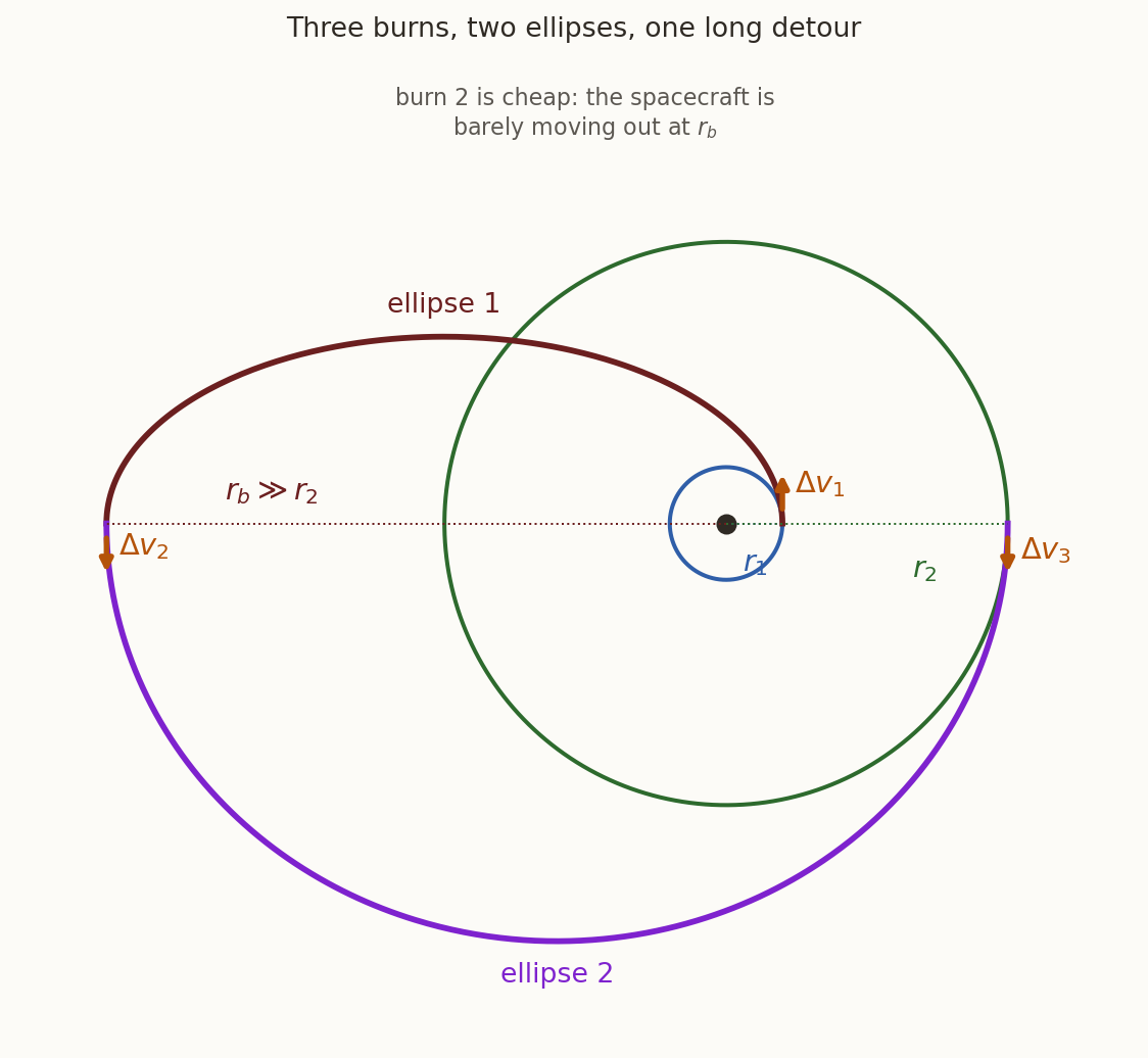
Figure 1 shows the route between a circle of radius \(r_1\), in blue, and a circle of radius \(r_2\), in green. It has three burns.
- Burn 1, at \(r_1\), puts the spacecraft on ellipse 1, in maroon, whose apoapsis is at a distant radius \(r_b>r_2\).
- Burn 2, at \(r_b\), puts it on ellipse 2, in purple, which has the same apoapsis and has its periapsis at \(r_2\). This burn raises the periapsis from \(r_1\) to \(r_2\).
- Burn 3, at \(r_2\), slows it down onto the circle. This burn is retrograde, because the spacecraft reaches \(r_2\) at the periapsis of ellipse 2, where it is moving faster than the circular speed.
Why should burn 2 be cheap? At an apsis the speed is \(v=h/r\), so a burn there costs \(\Delta v=\Delta h/r\). The angular momentum \(h\) fixes the periapsis of an orbit with a given apoapsis. So raising the periapsis means adding a certain amount of \(h\), and at a large \(r_b\) this costs only a small \(\Delta v\).
1.1.1 The cost of the three burns
On an ellipse with apsides at \(r\) and \(r'\), vis-viva gives the speed at \(r\) as
\[ v=\sqrt{\frac{2\mu r'}{r(r+r')}} . \]
We apply this to the two ellipses, with \(R=r_2/r_1\) and \(R^{*}=r_b/r_1\), so that \(R^{*}>R\). At \(r_1\) on ellipse 1 the speed is \(v_{c1}\sqrt{2R^{*}/(1+R^{*})}\), so the first burn is
\[ \frac{\Delta v_1}{v_{c1}}=\sqrt{\frac{2R^{*}}{1+R^{*}}}-1 . \]
At \(r_b\) the speed on ellipse 1 is \(v_{c1}\sqrt{2/(R^{*}(1+R^{*}))}\) and the speed on ellipse 2 is \(v_{c1}\sqrt{2R/(R^{*}(R+R^{*}))}\). The second burn is the difference, and both speeds contain the factor \(\sqrt{2/R^{*}}\).
\[ \frac{\Delta v_2}{v_{c1}}=\sqrt{\frac2{R^{*}}}\left(\sqrt{\frac{R}{R+R^{*}}}-\sqrt{\frac1{1+R^{*}}}\right). \]
At \(r_2\) the speed on ellipse 2 is \(v_{c1}\sqrt{2R^{*}/(R(R+R^{*}))}\) and the circular speed is \(v_{c1}/\sqrt R\). So the third burn, which is retrograde, has the size
\[ \frac{\Delta v_3}{v_{c1}}=\sqrt{\frac{2R^{*}}{R(R+R^{*})}}-\frac1{\sqrt R} . \tag{1}\]
Two things stand out. First, the factor \(\sqrt{2/R^{*}}\) in \(\Delta v_2\) makes it tend to zero as \(r_b\to\infty\). So in the limit, moving the periapsis by any amount costs nothing. Second, if we set \(R^{*}=R\), then \(\Delta v_3=0\) and the first two burns become the Hohmann transfer. So the bi-elliptic transfers are a family that starts at the Hohmann transfer and moves away from it as \(r_b\) grows.
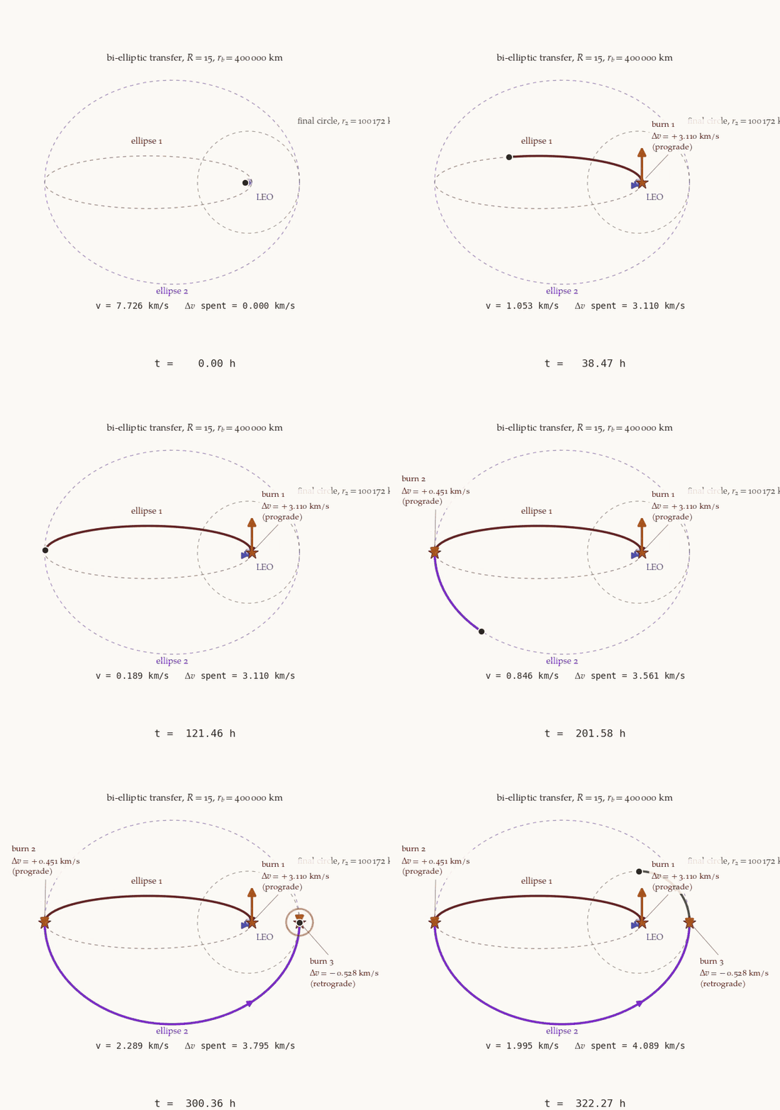
Example. A spacecraft is on a circle of radius \(r_1=6678.137\) km and must reach a circle of radius \(r_2=100\,172.06\) km, so that \(R=15\). Take \(\mu=398\,600.4418\) km\(^3\)/s\(^2\). For a bi-elliptic transfer with \(r_b=400\,000\) km, find the three burns, the total and the transfer time. Compare them with the Hohmann transfer.
Solution. The two ellipses have \(a_{t1}=(r_1+r_b)/2=203\,339\) km and \(a_{t2}=(r_2+r_b)/2=250\,086\) km. The speeds, in km/s, are as follows.
| Burn | Where | Speed before | Speed after | \(\Delta v\) |
|---|---|---|---|---|
| 1 | \(r_1\) | \(7.72576\) | \(10.83580\) | \(3.11004\) |
| 2 | \(r_b\) | \(0.18091\) | \(0.63178\) | \(0.45088\) |
| 3 | \(r_2\) | \(2.52279\) | \(1.99478\) | \(0.52801\) |
The total is \(4.08892\) km/s. The Hohmann transfer costs \(g(15)\,v_{c1}=4.14269\) km/s. So the bi-elliptic transfer saves \(53.8\) m/s, which is \(1.3\%\). The time is half a period of each ellipse added together, which is \(299.6\) h, or \(12.5\) days. The Hohmann transfer takes \(17.1\) h.
Burn 2 raises the periapsis by more than \(93\,000\) km for only \(0.45\) km/s, because the spacecraft is moving at only \(181\) m/s at \(r_b\).
Is this saving worth having? With \(I_{sp}=320\) s, the bi-elliptic transfer leaves \(27.2\%\) of the starting mass and the Hohmann transfer leaves \(26.7\%\). That is \(1.7\%\) more mass delivered, and the price is about \(12\) extra days of flight. There is also a caution. Our \(r_b\) is beyond the orbit of the Moon, and out there the pull of the Moon and the Sun is no longer a small correction. So the two-body numbers above would need checking against a better model before anyone relied on a saving of this size.
1.2 The two thresholds
When does the bi-elliptic transfer win? There are two different questions here, with two different answers.
Does the limiting case \(r_b\to\infty\) beat Hohmann? As \(R^{*}\to\infty\), the first burn tends to \(\sqrt2-1\), the second tends to \(0\), and the third tends to \(\sqrt{2/R}-1/\sqrt R=(\sqrt2-1)/\sqrt R\). So
\[ \frac{\Delta v_{\rm bi,\infty}}{v_{c1}}=(\sqrt2-1)\left(1+\frac1{\sqrt R}\right). \]
Setting this equal to \(g(R)\) and solving numerically gives
\[ \boxed{\;R^{\dagger}=11.938765 .\;} \]
Does every \(r_b>r_2\) beat Hohmann? For this we look at the family near its start at \(R^{*}=R\). Let \(C(R,R^{*})\) be the total cost in units of \(v_{c1}\). If \(C\) falls as \(R^{*}\) moves up from \(R\), then a small detour beyond the target already saves propellant. So we want the sign of \(\partial C/\partial R^{*}\) at \(R^{*}=R\).
There is a neat way to find this. We know that \(C(R,R)=g(R)\), because at \(R^{*}=R\) the transfer is the Hohmann transfer. Differentiating this with respect to \(R\) by the chain rule gives
\[ \left.\frac{\partial C}{\partial R}\right|_{R^{*}=R}+\left.\frac{\partial C}{\partial R^{*}}\right|_{R^{*}=R}=\frac{dg}{dR} . \]
Now we compute \(\partial C/\partial R\). Only burns 2 and 3 contain \(R\). Differentiating them and then setting \(R^{*}=R\) gives
\[ \begin{aligned} \frac{\partial}{\partial R}\left[\sqrt{\frac2{R^{*}}}\sqrt{\frac{R}{R+R^{*}}}\right]_{R^{*}=R}&=\frac1{4R^{3/2}},\\ \frac{\partial}{\partial R}\left[\sqrt{\frac{2R^{*}}{R(R+R^{*})}}-\frac1{\sqrt R}\right]_{R^{*}=R}&=-\frac1{4R^{3/2}}. \end{aligned} \]
These cancel, so \(\partial C/\partial R=0\) at \(R^{*}=R\), and therefore
\[ \left.\frac{\partial C}{\partial R^{*}}\right|_{R^{*}=R}=\frac{dg}{dR} . \]
This is a pleasing result. A detour beyond \(r_2\) saves propellant exactly when the Hohmann cost is falling with \(R\). The Hohmann note showed that this happens beyond the maximum of the Hohmann curve, so the second threshold is the same number.
\[ \boxed{\;R^{\ddagger}=15.581719 .\;} \]
The derivative tells us only what happens near \(R^{*}=R\). To say that every \(r_b>r_2\) wins, we also need the cost never to come back above Hohmann’s for larger \(r_b\). This is the classical result of Ting (1960). The verify script confirms it by a scan over \(15.6\le R\le100\) and \(R<r_b/r_1\le10^4\), and confirms by a similar scan that Hohmann always wins for \(R<11.94\). So there are three regions.
| Radius ratio | Which is cheaper |
|---|---|
| \(R<11.94\) | Hohmann, for every \(r_b\) |
| \(11.94<R<15.58\) | the bi-elliptic, but only if \(r_b\) is large enough |
| \(R>15.58\) | the bi-elliptic, for every \(r_b>r_2\) |
History: the bi-elliptic transfer. It was analysed by Ary Sternfeld in the 1930s and again, independently, in the late 1950s.
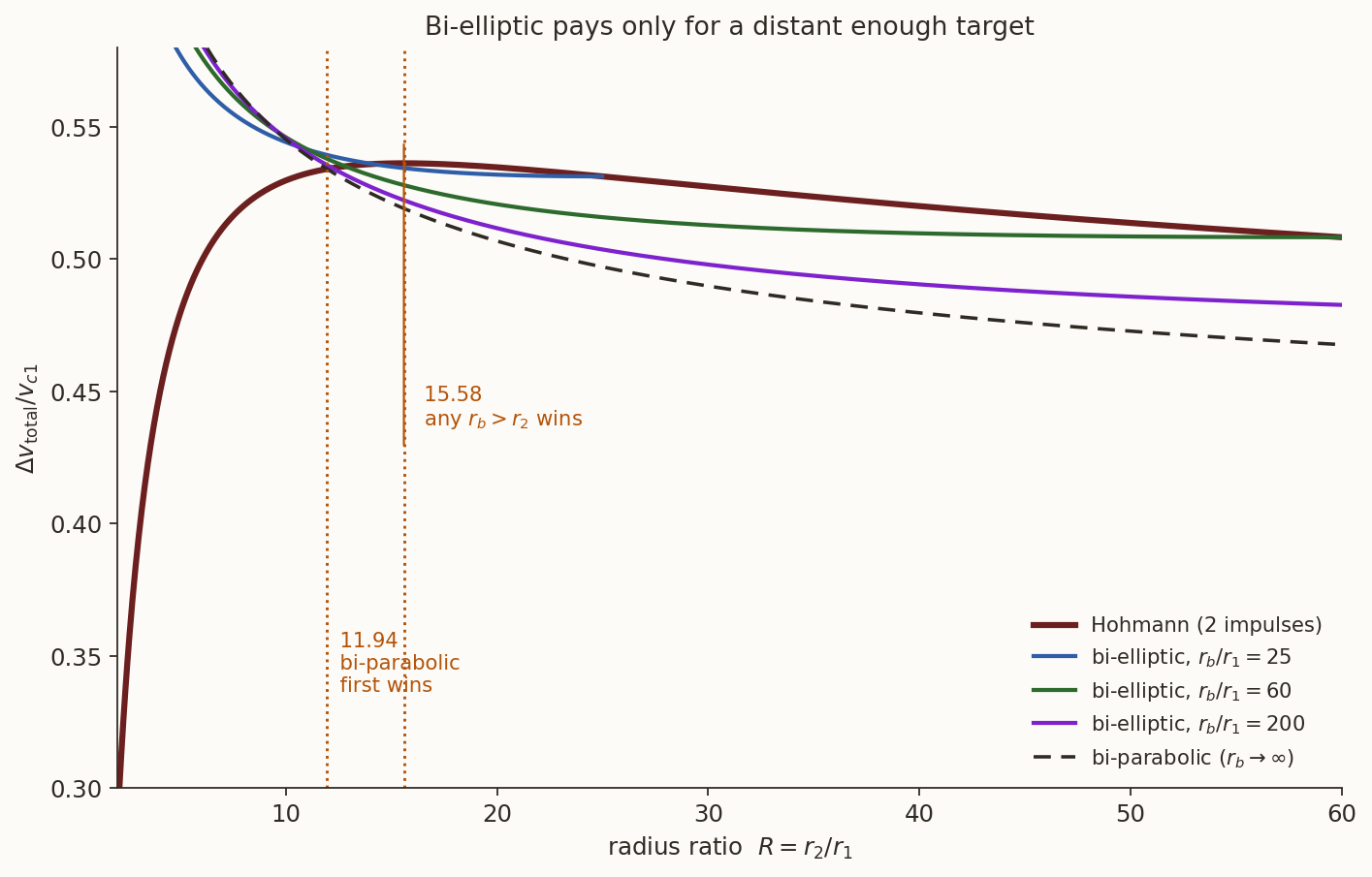
Figure 3 shows these regions. The maroon curve is Hohmann, the coloured curves are bi-elliptic transfers with a fixed \(r_b/r_1\), and the dashed curve is the limit \(r_b\to\infty\). The vertical lines mark the two thresholds.
The curve for \(r_b=25r_1\) looks as if it merges with Hohmann, but it does not. Between \(R=14.10\) and \(R=25\) it lies below Hohmann, by at most \(0.0030\,v_{c1}\), which is \(0.56\%\), near \(R=18.5\). The two meet only at \(R=25\), where \(r_b=r_2\) and the bi-elliptic transfer is the Hohmann transfer.
The transfer from a \(300\) km circle (\(r_1=6678.137\) km) to the geostationary orbit (\(r_2=42\,164\) km) has \(R=6.31\). Is the bi-elliptic transfer useful for putting satellites there?
Answer
No. \(R=6.31\) is well below \(11.94\), so Hohmann wins whatever \(r_b\) we choose.So the bi-elliptic transfer can help only for large \(R\), and even then it saves only a percent or two, at the cost of days or weeks. For a real mission the case for it is weak.
1.3 A stopover is not a bi-elliptic
What if the middle burn is made short of the target, with \(r_b<r_2\)? This is still a three-impulse manoeuvre, and we might hope that it also saves something. We will show that it never does.
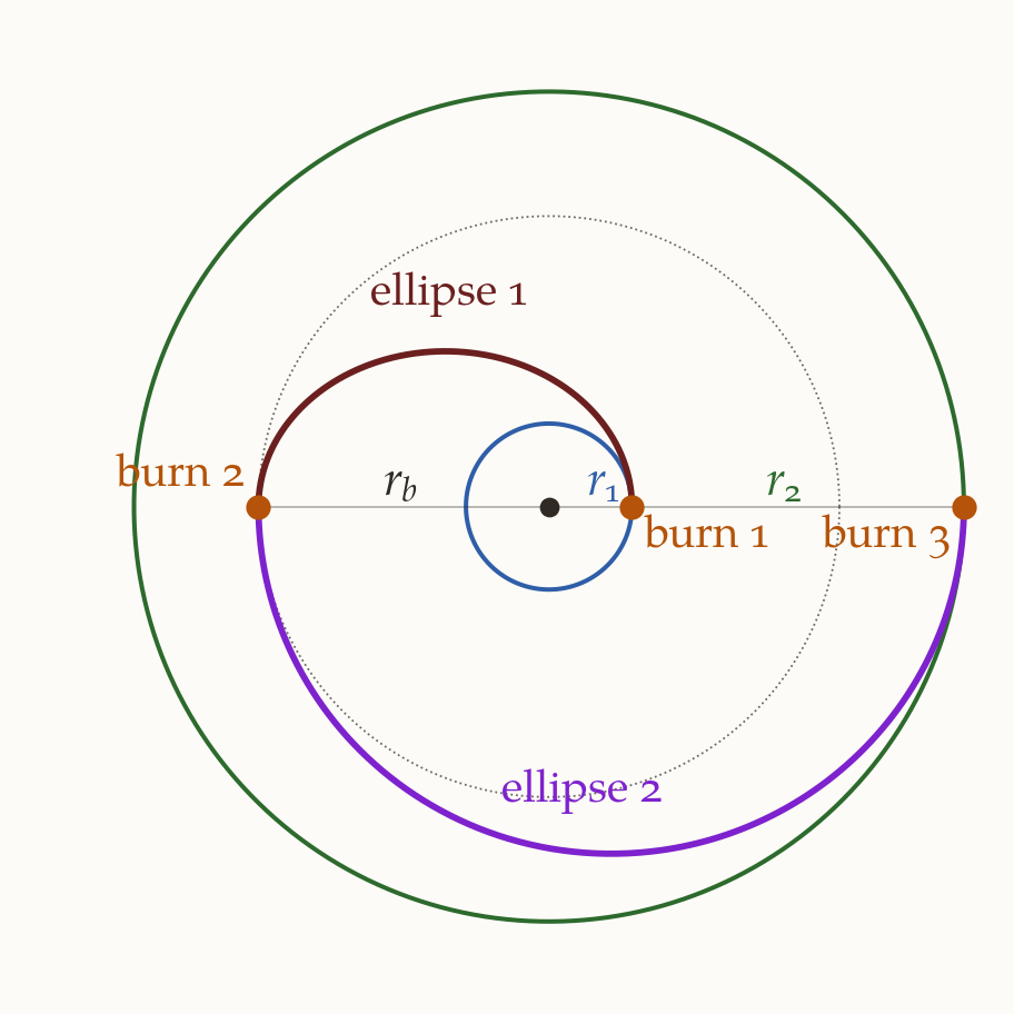
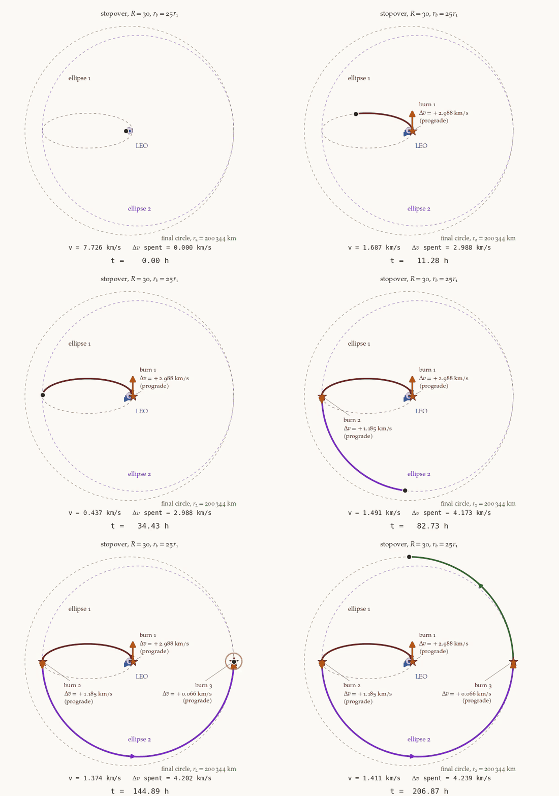
Figure 4 shows the route. Ellipse 1, in maroon, climbs from \(r_1\) to \(r_b\). Ellipse 2, in purple, now runs from its periapsis at \(r_b\) out to its apoapsis at \(r_2\). This changes two things compared with the bi-elliptic transfer. Burn 2 now has to raise the apoapsis, which means adding energy at low speed. And the spacecraft reaches \(r_2\) below the circular speed, so burn 3 is prograde, with the size
\[ \frac{\Delta v_3}{v_{c1}}=\frac1{\sqrt R}-\sqrt{\frac{2R^{*}}{R(R+R^{*})}}\qquad(R^{*}<R). \]
This is minus the expression in Equation 1. If we added up that formula blindly here, we would subtract the third burn instead of adding it.
Example. A spacecraft on a circle of radius \(r_1=6678.137\) km must reach a circle with \(R=30\). It uses a stopover at \(r_b=25r_1\). Take \(\mu=398\,600.4418\) km\(^3\)/s\(^2\). Find the three burns, the total and the time, and compare them with the Hohmann transfer. Burn 1 turns out to be cheaper than the first burn of the Hohmann transfer. So where does the extra cost come from?
Solution. The radii are \(r_2=200\,344.11\) km and \(r_b=166\,953.43\) km. The ellipses have \(a_{t1}=86\,815.78\) km and \(a_{t2}=183\,648.77\) km. The speeds, in km/s, are as follows.
| Burn | Where | Speed before | Speed after | \(\Delta v\) |
|---|---|---|---|---|
| 1 | \(r_1\) | \(7.72576\) | \(10.71370\) | \(2.98794\) |
| 2 | \(r_b\) | \(0.42855\) | \(1.61386\) | \(1.18531\) |
| 3 | \(r_2\) | \(1.34488\) | \(1.41052\) | \(0.06564\) |
The total is \(4.23889\) km/s and the time is \(6.01\) days. The Hohmann transfer costs \(4.07470\) km/s and takes \(1.92\) days. So the stopover costs \(4.03\%\) more and takes about three times as long.
Burn 1 saves \(34.5\) m/s compared with the Hohmann first burn of \(3.02245\) km/s, because it does not climb the last \(33\,391\) km. But burns 2 and 3 together then cost \(198.7\) m/s more than the Hohmann arrival burn. The missing energy has to be added at \(r_b\), where the spacecraft moves at \(0.429\) km/s, and not at \(r_1\), where it moved at \(10.71\) km/s. By conservation of angular momentum the ratio of these two speeds is exactly \(r_b/r_1=25\). So there each m/s adds \(25\) times less energy.
The result of this example holds generally. At both ends of the range of \(r_b\) the stopover is the Hohmann transfer, because \(R^{*}=1\) puts the middle burn at \(r_1\) and \(R^{*}=R\) circularises on arrival. Everything in between costs more. For \(R=30\) the worst choice is \(R^{*}=4.02\), which costs \(34\%\) more than Hohmann.
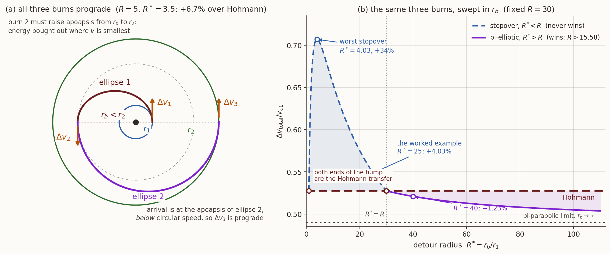
Figure 6 shows the whole picture for \(R=30\) in its right panel. The hump on the left is the stopover. To the right of \(R^{*}=30\) the curve falls below Hohmann. With \(r_b=40r_1\), for example, the same three-burn structure costs \(4.02458\) km/s, which is \(1.2\%\) less than Hohmann. Since \(R=30\) is above \(15.58\), this is what we expected.
Why is one direction so much better than the other? In the bi-elliptic transfer the far burn changes the periapsis, which costs little at low speed because it needs a change of \(h\). In the stopover the far burn has to add energy, and energy is expensive at low speed. So it is the same low speed that helps in one case and hurts in the other.
The practical lesson is that a mission should not break a transfer into an intermediate waiting orbit in the hope of saving propellant. A parking orbit on the way can be useful for other reasons, such as waiting for the right time to leave, but it will cost \(\Delta v\).
2 Summary and exercises
The bi-elliptic transfer goes beyond the target and comes back, using three burns. It beats Hohmann for \(R>11.94\) with a large enough \(r_b\), and for every \(r_b>r_2\) when \(R>15.58\), which is the maximum of the Hohmann curve. The saving is small and the extra time is large. A stopover, with \(r_b<r_2\), is always worse than Hohmann.
- Moon transfer. Compute the Hohmann \(\Delta v\) and the transfer time from a circle of radius \(r_1=6678.137\) km to a circular orbit of radius \(384\,400\) km, ignoring the Moon’s gravity and taking \(\mu=398\,600.4418\) km\(^3\)/s\(^2\). Would a bi-elliptic transfer help? (Answers: \(3.106+0.830=3.937\) km/s in \(4.98\) days. \(R=57.6>15.58\), so yes in principle. Taking \(r_b=2r_2\) saves \(133\) m/s but takes \(39\) days, and the limit \(r_b\to\infty\) saves at most \(315\) m/s. Any \(r_b\) much beyond \(2r_2\) also leaves the Earth’s sphere of influence, so the model fails there. ISRO’s Chandrayaan missions reach the Moon differently, as the Indian missions problems show. They build up the orbit in steps, with a series of burns near perigee.)
All the numbers in this note are checked by bielliptic-transfer-verify.py.