The Hohmann Transfer
1 The Hohmann transfer
Suppose a spacecraft is on a circular orbit and we want to move it to a larger circular orbit in the same plane. This is the most common task in orbital manoeuvring. A communication satellite launched from Sriharikota, for example, has to end up on the geostationary orbit, far above the height at which its launch begins.
We change an orbit by firing a rocket engine. In this note we treat each firing as an impulse, which is a sudden change of the velocity at a fixed position. This is a good model when the burn is short compared with the orbital period. The cost of an impulse is the size of the change, \(\Delta v=|\mathbf v^+-\mathbf v^-|\), where \(\mathbf v^-\) and \(\mathbf v^+\) are the velocities just before and just after it. The cost of a sequence of impulses is the sum of these sizes. The propellant needed grows exponentially with this total, as the rocket equation shows, so we look for the route with the smallest total \(\Delta v\).
We will first find a good route between two circles and work out its cost. We will then ask how the cost changes as the target moves farther away. After that we will move from circles to ellipses, which have more than one route, and to orbits that cross. Finally we will prove that no other two-impulse transfer between two circles is cheaper than the one we found.
1.1 From one circle to another
Let the two circles have radii \(r_1<r_2\). An impulse changes the velocity but not the position. So one impulse can move a spacecraft from one orbit to another only at a point that lies on both. Two circles of different radii have no point in common, so one impulse is not enough. We need at least two, with a transfer orbit between them that reaches both circles.
Many conics reach both circles, so which one should we choose? Consider the first burn. Just before it the spacecraft has the circular speed \(v_c\), and just after it the transfer speed \(v\). If the angle between the two velocities is \(\phi\), the law of cosines gives
\[ \Delta v^2=v^2+v_c^2-2vv_c\cos\phi . \]
For given speeds this is smallest when \(\phi=0\), and then \(\Delta v=|v-v_c|\). Any other angle pays extra for turning the velocity. So we want the velocity on the transfer orbit to be parallel to the velocity on the circle at both burns.
On a circle, the velocity is always perpendicular to the radius. On an ellipse, this is true at only two points, the periapsis and the apoapsis. We therefore place the periapsis of the transfer ellipse on the inner circle and its apoapsis on the outer circle. Exactly one ellipse does this, and it touches each circle at one point. This is the Hohmann transfer.
So far this is only a good reason to try this ellipse, not a proof that it is the best. We will give the proof in Section 1.5.
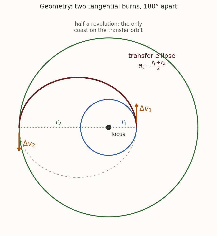
Figure 1 shows the route. The inner circle is blue and the outer circle is green. The first burn, \(\Delta v_1\), puts the spacecraft on the transfer ellipse in maroon. It then coasts along half of the ellipse, and the second burn, \(\Delta v_2\), puts it on the outer circle.
1.1.1 The cost of the transfer
The major axis of the ellipse runs from \(r_1\) to \(r_2\), so \(a_t=(r_1+r_2)/2\). We substitute this in vis-viva, \(v^2=\mu(2/r-1/a)\), to find the speed at each end of the ellipse. At \(r_1\),
\[ v_{t1}^2=\mu\left(\frac2{r_1}-\frac2{r_1+r_2}\right)=\frac{2\mu r_2}{r_1(r_1+r_2)}, \]
and in the same way at \(r_2\),
\[ v_{t2}^2=\mu\left(\frac2{r_2}-\frac2{r_1+r_2}\right)=\frac{2\mu r_1}{r_2(r_1+r_2)}. \]
Both burns are along the velocity, so each one costs a difference of speeds. The circular speeds are \(v_{c1}=\sqrt{\mu/r_1}\) and \(v_{c2}=\sqrt{\mu/r_2}\), so
\[ \boxed{\;\begin{aligned} \Delta v_1&=v_{t1}-v_{c1}=\sqrt{\frac{\mu}{r_1}}\left(\sqrt{\frac{2r_2}{r_1+r_2}}-1\right),\\ \Delta v_2&=v_{c2}-v_{t2}=\sqrt{\frac{\mu}{r_2}}\left(1-\sqrt{\frac{2r_1}{r_1+r_2}}\right). \end{aligned}\;} \tag{1}\]
Since \(r_2>r_1\), we have \(2r_2/(r_1+r_2)>1\) and \(2r_1/(r_1+r_2)<1\). So both of these are positive and both burns add speed.
The spacecraft flies half of the ellipse, so the transfer takes half of its period.
\[ t_{\rm H}=\pi\sqrt{\frac{a_t^3}{\mu}} . \]
History: Hohmann. Walter Hohmann, a German civil engineer, published this transfer in 1925 in Die Erreichbarkeit der Himmelskörper (“The attainability of the heavenly bodies”), decades before any spacecraft flew.
Example. A spacecraft is on a circular orbit at \(300\) km altitude, with radius \(r_1=6678.137\) km. It has to reach the geostationary orbit, a circle of radius \(r_2=42\,164\) km. Take \(\mu=398\,600.4418\) km\(^3\)/s\(^2\). For the Hohmann transfer, find the semi-major axis and the eccentricity of the transfer ellipse, the two impulses, their total and the transfer time. Is each burn along the motion (prograde) or against it (retrograde)?
Solution. The transfer ellipse has
\[ a_t=\frac{6678.137+42\,164}{2}=24\,421.07\text{ km},\qquad e_t=\frac{r_2-r_1}{r_2+r_1}=0.72654 . \]
The formulas above give the following speeds, in km/s.
| Speed before | Speed after | \(\Delta v\) | |
|---|---|---|---|
| Burn 1, at \(r_1\) | \(v_{c1}=7.72576\) | \(v_{t1}=10.15149\) | \(2.42573\) |
| Burn 2, at \(r_2\) | \(v_{t2}=1.60784\) | \(v_{c2}=3.07467\) | \(1.46682\) |
The total is \(3.89255\) km/s. The transfer time is \(t_{\rm H}=\pi\sqrt{24\,421.07^3/398\,600.4418}=18\,990\) s, which is \(5.275\) h. Both burns are prograde, because each one raises the speed.
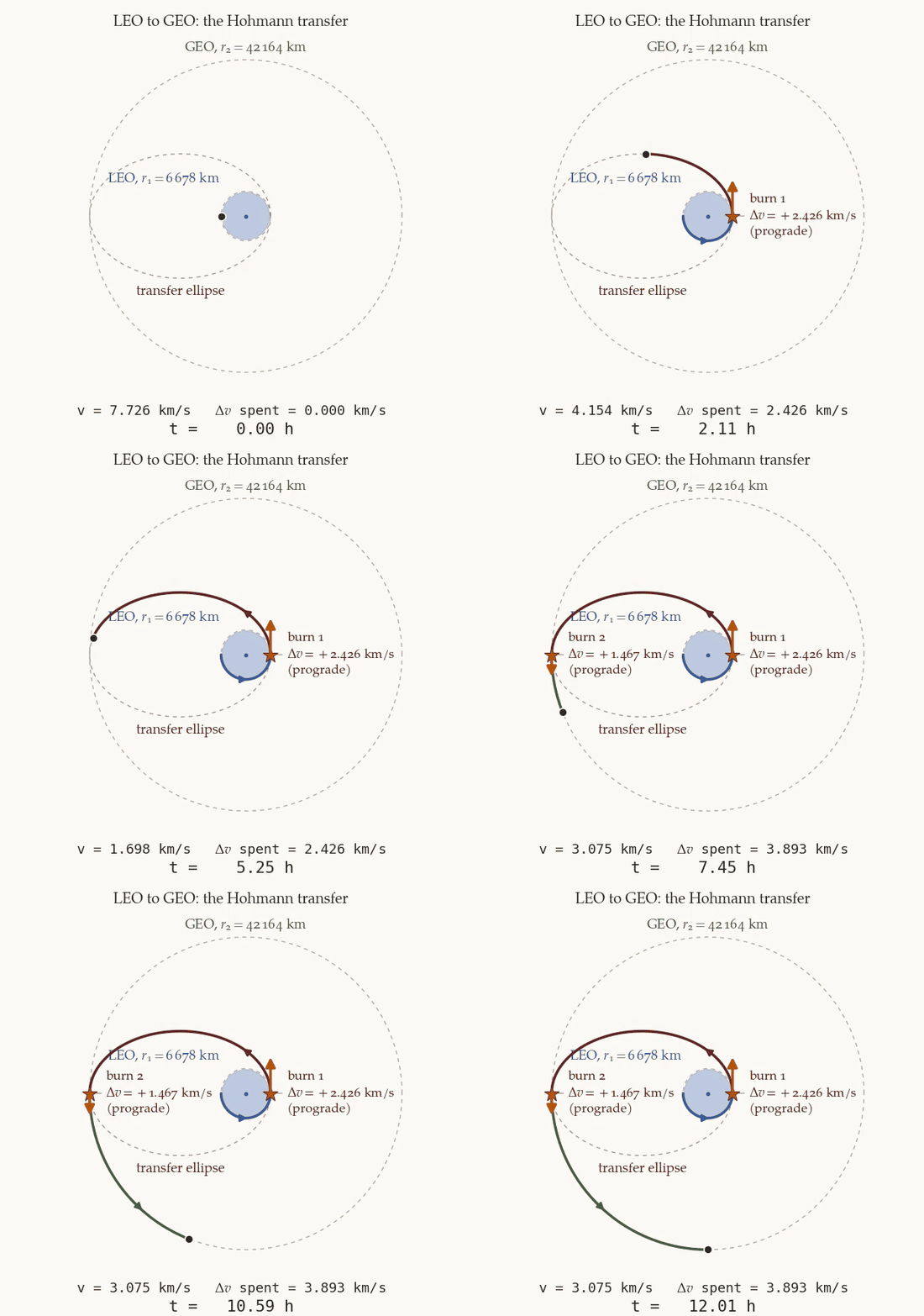
There is something surprising in the table. The spacecraft ends up slower on the outer circle (\(3.07\) km/s) than it was on the inner circle (\(7.73\) km/s), and yet both burns add speed. This works because the coast takes away much more speed than the burns add. Between the two burns the speed falls from \(10.15\) km/s to \(1.61\) km/s, as kinetic energy turns into potential energy.
What does this cost a real mission? With the rocket equation and \(I_{sp}=320\) s, which is typical of the storable propellants that satellites use, a total of \(3.893\) km/s would leave only \(28.9\%\) of the starting mass. Less than a third of the mass would be left for the satellite itself, its tanks and its engine. So the two burns are normally shared out. The upper stage of the launcher, which is built for large burns, makes something like the first burn. It leaves the satellite on a transfer ellipse. The satellite then makes the second burn with its own engine. That burn alone leaves \(62.7\%\) of the mass, which is far more practical. In a real launch from Sriharikota this second burn also has to turn the orbital plane, as the plane-changes note explains.
1.2 A farther target can cost less
How does the cost change as the target moves farther away? It seems obvious that it must keep growing. To test this, we measure the cost in units of \(v_{c1}\), the speed we start with, and write \(R=r_2/r_1\). Then \(\sqrt{\mu/r_2}=v_{c1}/\sqrt R\), and Equation 1 becomes
\[ \frac{\Delta v_{\rm H}}{v_{c1}}=g(R)= \underbrace{\sqrt{\frac{2R}{1+R}}-1}_{\text{departure}} +\underbrace{\frac1{\sqrt R}\left(1-\sqrt{\frac2{1+R}}\right)}_{\text{arrival}} . \tag{2}\]
For \(g(R)=\sqrt{2R/(1+R)}-1+\left(1-\sqrt{2/(1+R)}\right)/\sqrt R\), evaluate \(g\) at \(R=6.31\), \(R=15\), \(R=100\) and in the limit \(R\to\infty\). What do you notice?
What you should find
\(g(6.31)=0.5038\), \(g(15)=0.5362\), \(g(100)=0.4931\) and \(g(\infty)=\sqrt2-1=0.4142\). The cost rises and then falls. A target \(100\) times farther away than the start is cheaper to reach than one \(15\) times farther away.Why does the cost fall? Consider the two terms of Equation 2 separately as \(R\) grows.
The departure term keeps rising, but it approaches a limit, \(\sqrt2-1\). This limit is the escape burn, because \(\sqrt{2\mu/r_1}-\sqrt{\mu/r_1}=(\sqrt2-1)v_{c1}\). So going very far costs almost as much as leaving for good, and no more than that.
The arrival term has a factor \(1/\sqrt R\), because the arrival burn has to match the circular speed of the target, and this speed falls as the target moves away. So for large \(R\) the arrival term falls to zero.
At large \(R\), then, the departure term has almost stopped growing while the arrival term keeps shrinking. So the total must have a maximum. To find it, we differentiate Equation 2 term by term.
\[ \frac{dg}{dR}=\frac{1}{\sqrt{2R}\,(1+R)^{3/2}}-\frac{1}{2R^{3/2}}+\frac{1+2R}{\sqrt2\,R^{3/2}(1+R)^{3/2}} . \]
We set this to zero and multiply through by \(\sqrt2\,R^{3/2}(1+R)^{3/2}\), which gives
\[ R-\frac{(1+R)^{3/2}}{\sqrt2}+1+2R=0, \qquad\text{that is}\qquad \sqrt2\,(1+3R)=(1+R)^{3/2} . \]
Squaring both sides and collecting terms gives a cubic equation.
\[ 2(1+3R)^2=(1+R)^3 \qquad\Longrightarrow\qquad R^3-15R^2-9R-1=0 . \]
This cubic has one positive root, which we find numerically. It gives
\[ \boxed{\;\max_R g(R)=0.536258\quad\text{at}\quad R=15.581719 .\;} \tag{3}\]
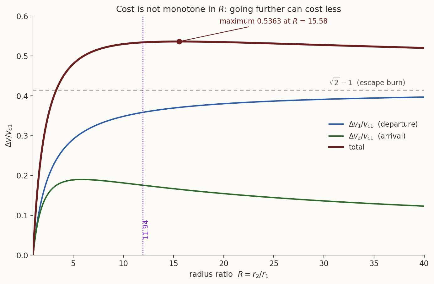
Figure 3 shows the result. The blue curve is the departure burn and it rises towards the dashed line, which is the escape burn. The green curve is the arrival burn and it falls after a small rise. The maroon curve is the total, with its maximum at \(R=15.58\).
This has a practical meaning. Since \(g\) never exceeds \(0.536258\), a spacecraft starting from our \(300\) km circle with \(v_{c1}=7.726\) km/s can reach any circular orbit about the Earth in its plane for at most \(4.143\) km/s. But we should be careful about what this does not say. The time does keep growing with the distance. It is \(5.3\) h to the geostationary orbit and about \(5\) days to the distance of the Moon. Far from the Earth a long coast also leaves more time for small errors and for the pull of other bodies to matter. So a cheap distant target is not necessarily an easy one.
1.3 Between two ellipses with a common apse line
Real orbits are rarely circular. Suppose both orbits are ellipses in the same plane, and they share a line of apsides. We say that such orbits are coaxial. What is the cheapest way from the inner one to the outer one?
We use the same argument as for the circles. A burn is cheapest when the velocities before and after it are parallel. The transfer ellipse has its velocity perpendicular to the radius only at its two apsides, and the same is true of each orbit. So the burns should be made where an apsis of the transfer ellipse meets an apsis of the orbit. The two apsides of an ellipse are on opposite sides of the focus. So the candidates are half-ellipses from an apsis of orbit 1 to the apsis of orbit 2 on the opposite side. There are always two of these, so a new question arises. Which one is cheaper?
1.3.1 Aligned apsides
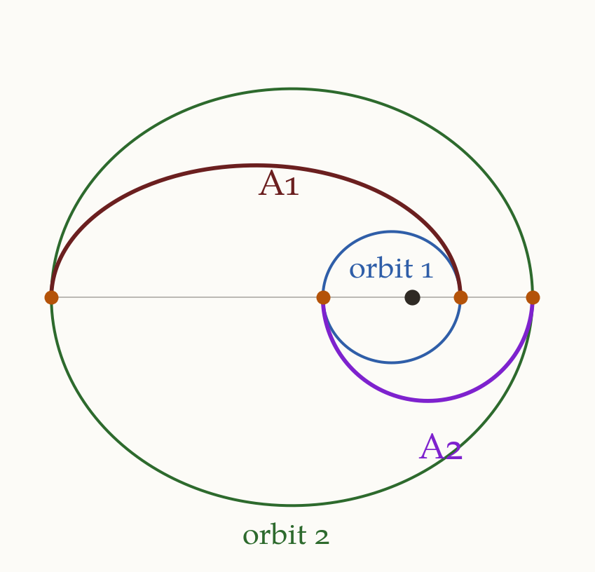
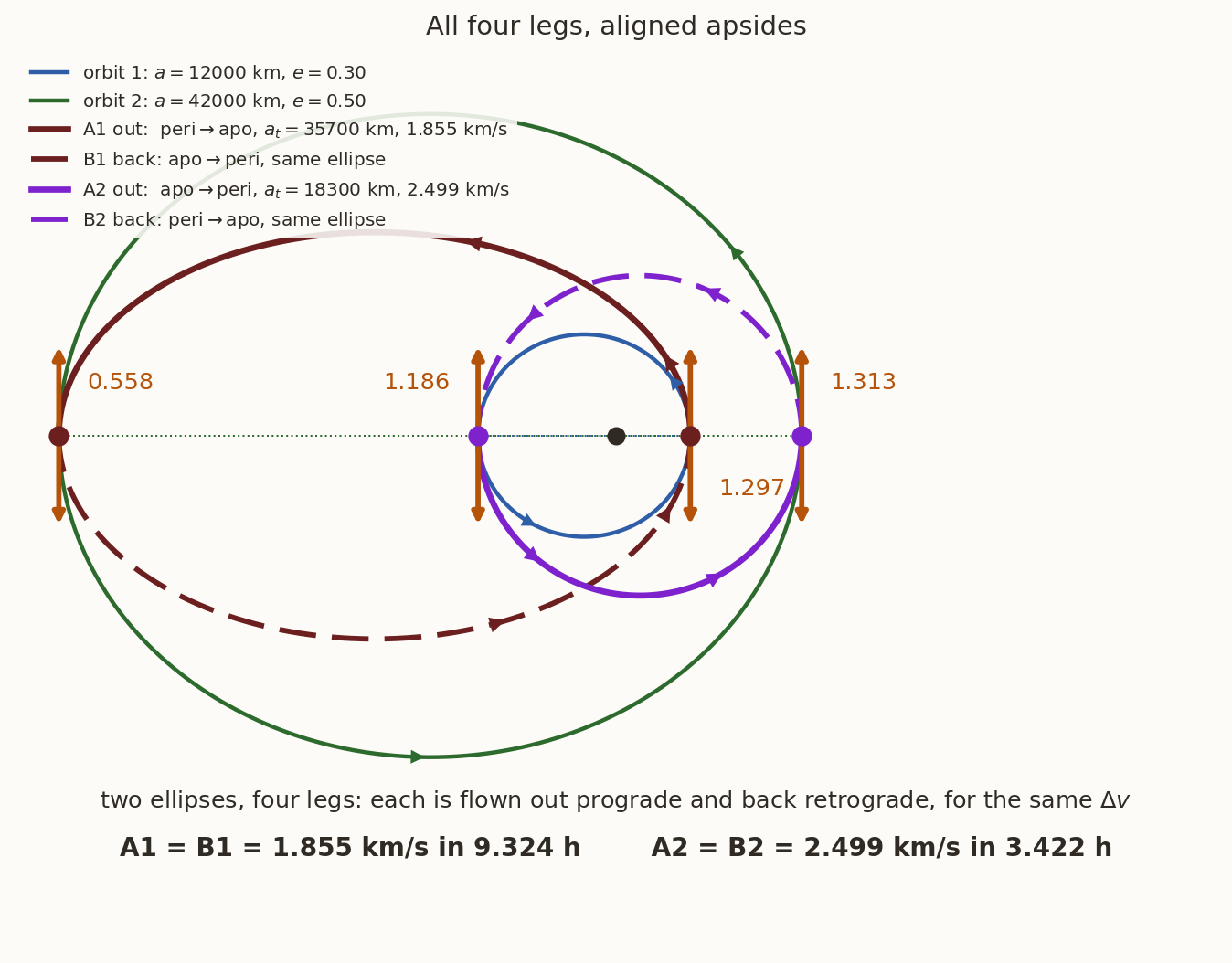
In Figure 4 the two periapses point the same way, to the right of the focus. Route A1, in maroon, joins the periapsis of orbit 1 to the apoapsis of orbit 2. Route A2, in purple, joins the apoapsis of orbit 1 to the periapsis of orbit 2. Their semi-major axes are
\[ \text{A1}:\ a_t=\frac{r_{p,1}+r_{a,2}}{2},\qquad \text{A2}:\ a_t=\frac{r_{a,1}+r_{p,2}}{2}. \]
Each impulse is the difference between the speed on the transfer ellipse and the speed on the orbit at that point. Both come from vis-viva, so
\[ \Delta v=\left|\sqrt{\mu\left(\frac2r-\frac1{a_t}\right)}-\sqrt{\mu\left(\frac2r-\frac1{a_{\rm orbit}}\right)}\right| . \]
Can we predict the winner without calculating? Both routes have to add the same total energy, the difference between the energies of the two orbits. A burn \(\Delta v\) along a velocity \(v\) adds the specific energy
\[ \Delta\varepsilon=\frac12(v+\Delta v)^2-\frac12v^2=v\,\Delta v+\frac12\Delta v^2 . \]
So the same \(\Delta v\) adds more energy where the spacecraft is fast. This is called the Oberth effect. The cheaper route should therefore add as much of the energy as possible at high speed. Route A1 leaves orbit 1 at its periapsis, the fastest point of that orbit. It also reaches out as far as orbit 2 does, so the first burn adds nearly all of the energy and very little is left for the second burn. So we expect A1 to be the cheaper route.
Example. Orbit 1 has \(a_1=12\,000\) km and \(e_1=0.30\). Orbit 2 has \(a_2=42\,000\) km and \(e_2=0.50\). Their apsides are aligned, and \(\mu=398\,600.4418\) km\(^3\)/s\(^2\). Find the cost and the time of routes A1 and A2.
Solution. The radii of the apsides are \(r_{p,1}=8400\) km, \(r_{a,1}=15\,600\) km, \(r_{p,2}=21\,000\) km and \(r_{a,2}=63\,000\) km. Using these in the formulas above, with each transfer taking half a period, gives the following.
| \(a_t\) (km) | \(\Delta v_1\) (km/s) | \(\Delta v_2\) (km/s) | Total (km/s) | Time (h) | |
|---|---|---|---|---|---|
| A1, \(8400\to63\,000\) km | \(35\,700\) | \(1.29675\) | \(0.55850\) | \(1.85525\) | \(9.324\) |
| A2, \(15\,600\to21\,000\) km | \(18\,300\) | \(1.18573\) | \(1.31337\) | \(2.49909\) | \(3.422\) |
Route A1 is cheaper by \(644\) m/s, as we predicted. Route A2 is faster, by a factor of \(2.72\).
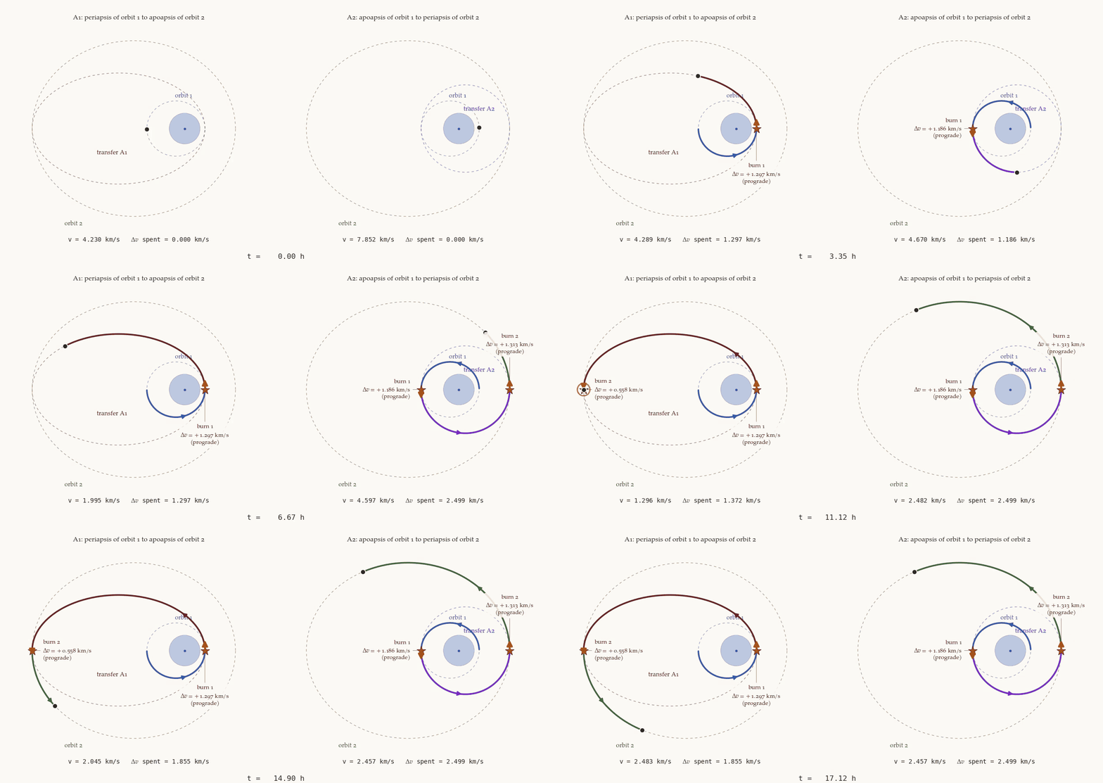
This is a real trade-off between propellant and time. With \(I_{sp}=320\) s, route A1 leaves \(55.4\%\) of the starting mass and route A2 leaves \(45.1\%\). So A1 delivers about \(23\%\) more mass, and A2 arrives about \(5.9\) h sooner. For most missions a few hours are worth far less than a quarter more spacecraft, so A1 would be the normal choice.
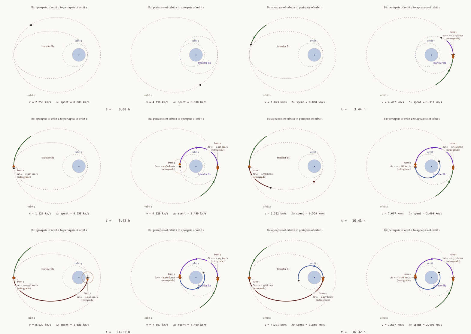
What about the return journey? The same two ellipses can be flown inward. Route B1 leaves the apoapsis of orbit 2 along the A1 ellipse and reaches the periapsis of orbit 1. Route B2 leaves the periapsis of orbit 2 along the A2 ellipse and reaches the apoapsis of orbit 1.
Orbit 1 and orbit 2 are as in the example, where the outward route A1 costs \(1.29675+0.55850\) km/s in \(9.324\) h and route A2 costs \(1.18573+1.31337\) km/s in \(3.422\) h. Without computing anything new, what do the return routes B1 and B2 cost, and how long do they take?
Answer
Exactly the same, with the two burns in the opposite order. Route B1 costs \(0.55850+1.29675=1.85525\) km/s in \(9.324\) h, and B2 costs \(1.31337+1.18573=2.49909\) km/s in \(3.422\) h. At each end the two speeds involved do not depend on the direction of travel, and \(|v_{\rm orbit}-v_t|=|v_t-v_{\rm orbit}|\). Only the sense of each impulse changes, from prograde to retrograde.This symmetry has a practical side. Going down also needs retrograde burns, and the atmosphere can supply a retrograde push without any propellant, whereas nothing natural supplies a prograde one. This is why aerobraking, which dips the orbit into the upper atmosphere and lets drag lower the apoapsis, can replace burns on the way down but never on the way up.
1.3.2 Anti-aligned apsides
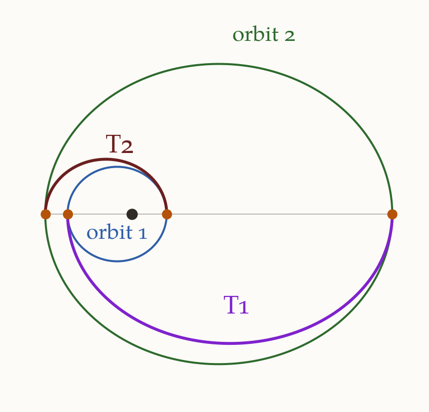
Now we turn orbit 2 through \(180^\circ\), so that its periapsis is on the opposite side, as in Figure 8. The two orbits have the same shapes as before. The transfer ellipses now join the periapses to each other, or the apoapses to each other. Route T2, in maroon, joins the periapses and route T1, in purple, joins the apoapses. Their semi-major axes are
\[ \text{T2}:\ a_t=\frac{r_{p,1}+r_{p,2}}{2},\qquad \text{T1}:\ a_t=\frac{r_{a,1}+r_{a,2}}{2}. \]
Example. Take the same orbits as in the previous example, with \(a_1=12\,000\) km, \(e_1=0.30\), \(a_2=42\,000\) km and \(e_2=0.50\), but with the apsides anti-aligned. Take \(\mu=398\,600.4418\) km\(^3\)/s\(^2\). Find the cost and the time of routes T2 and T1. Compare the cheaper route with route A1 of the aligned case, which cost \(1.855\) km/s.
Solution. The radii are the same as before, so the same formulas give the following.
| \(a_t\) (km) | \(\Delta v_1\) (km/s) | \(\Delta v_2\) (km/s) | Total (km/s) | Time (h) | |
|---|---|---|---|---|---|
| T2, \(8400\to21\,000\) km | \(14\,700\) | \(0.37924\) | \(2.04250\) | \(2.42174\) | \(2.464\) |
| T1, \(15\,600\to63\,000\) km | \(39\,300\) | \(2.17083\) | \(0.19386\) | \(2.36469\) | \(10.769\) |
Route T1 is cheaper, but only by \(57\) m/s, which is \(2.4\%\). Route T2 is \(4.37\) times faster. The cheaper route costs \(2.365\) km/s, against \(1.855\) km/s for the aligned orbits. So with the same two orbit shapes, the orientation alone adds \(27\%\) to the cost.
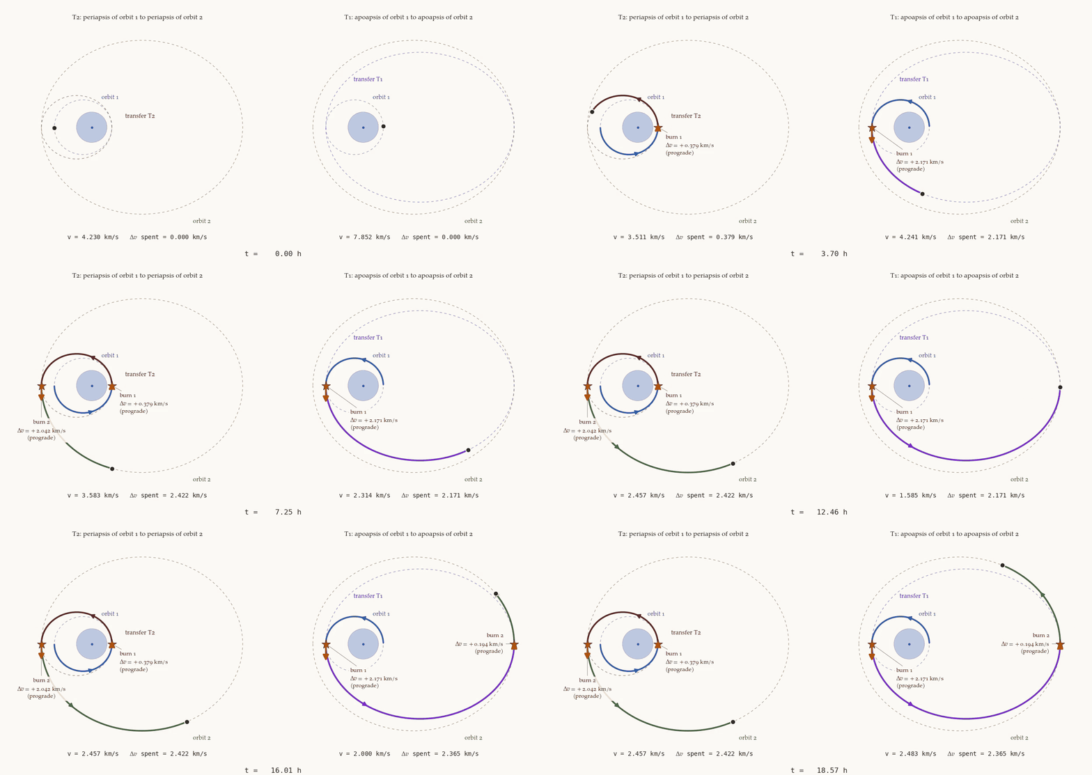
Here the trade-off looks very different. Route T1 saves only \(57\) m/s but takes \(8.3\) h longer, so a mission might well accept the extra cost of T2. The first lesson for a mission designer, though, is the \(27\%\). When we choose the starting orbit, it is worth choosing its apse line so that the orbits are aligned.
1.3.3 Which route is quicker, and which is cheaper?
Time has a simple answer. Each route is half a revolution of its transfer ellipse, so the route with the larger \(a_t\) is the slower one. Write \(c_i=a_ie_i\) for the distance from the centre of orbit \(i\) to its focus, so that \(r_{a,i}-r_{p,i}=2c_i\). With anti-aligned apsides,
\[ a_t^{\rm apo\to apo}-a_t^{\rm peri\to peri}=\frac{(r_{a,1}-r_{p,1})+(r_{a,2}-r_{p,2})}{2}=c_1+c_2 . \]
This is always positive, so the route joining the apoapses is always the slower. In the example, \(c_1+c_2=3600+21\,000=24\,600\) km, which is indeed \(39\,300-14\,700\) km. With aligned apsides,
\[ a_t^{\rm peri\to apo}-a_t^{\rm apo\to peri}=\frac{(r_{a,2}-r_{p,2})-(r_{a,1}-r_{p,1})}{2}=c_2-c_1 . \]
So the route from periapsis to apoapsis is the slower one only if the outer orbit has the larger \(c\).
Cost is less simple. Our argument for route A1 gives two rules. We should leave the inner orbit at its periapsis, and we should arrive at the outer orbit at its apoapsis.
With aligned apsides, route A1 obeys both rules. We prove below that it is always the cheaper route.
With anti-aligned apsides, the periapsis of orbit 1 and the apoapsis of orbit 2 are on the same side of the focus, so no half-ellipse joins them. Route T2 obeys the first rule and route T1 obeys the second. Which rule matters more depends on all four radii, as the next check shows.
Take \(a_1=12\,000\) km, \(a_2=42\,000\) km and \(e_2=0.50\) with anti-aligned apsides, as in the example, but raise \(e_1\) from \(0.30\) to \(0.45\). Take \(\mu=398\,600.4418\) km\(^3\)/s\(^2\). Which of the routes T2 and T1 is cheaper now?
Answer
Now \(r_{p,1}=6600\) km and \(r_{a,1}=17\,400\) km. Route T2 has \(a_t=13\,800\) km and costs \(0.22870+2.32292=2.55162\) km/s in \(2.241\) h. Route T1 has \(a_t=40\,200\) km and costs \(2.44215+0.12377=2.56592\) km/s in \(11.141\) h. So T2 is now cheaper, and it is still the faster one too. The order of cost has reversed.Proof that A1 always wins with aligned apsides. You can skip this proof on a first reading. Assume that orbit 1 lies inside orbit 2, so \(r_{p,1}<r_{p,2}\) and \(r_{a,1}<r_{a,2}\). Two facts make the algebra manageable.
The first fact is that at an apsis \(v=h/r\), so a tangential burn there costs \(|\Delta h|/r\).
The second fact is that a conic with apsidal radii \(r\) and \(r'\) has \(p=2rr'/(r+r')\). Using \(h=\sqrt{\mu p}\),
\[ h=\Phi\left(\frac1r+\frac1{r'}\right),\qquad\text{where}\quad\Phi(s)=\sqrt{\frac{2\mu}{s}} . \]
The radii enter only through their reciprocals, so we put \(x_i=1/r_{p,i}\) and \(y_i=1/r_{a,i}\). The hypotheses become \(x_1\ge y_1\), \(x_2\ge y_2\), \(x_1>x_2\) and \(y_1>y_2\). The function \(\Phi\) is decreasing and convex, which means \(\Phi'<0<\Phi''\). All four burns are prograde, so
\[ \begin{aligned} \Delta v_{A1}&=x_1\left[\Phi(x_1+y_2)-\Phi(x_1+y_1)\right]+y_2\left[\Phi(x_2+y_2)-\Phi(x_1+y_2)\right],\\ \Delta v_{A2}&=y_1\left[\Phi(y_1+x_2)-\Phi(x_1+y_1)\right]+x_2\left[\Phi(x_2+y_2)-\Phi(y_1+x_2)\right]. \end{aligned} \]
We subtract and collect the coefficient of each value of \(\Phi\). To write the result compactly, let \(L(\sigma,\tau)=(\sigma-\tau)\,\Phi(\sigma+\tau)\). This function is antisymmetric, \(L(\sigma,\tau)=-L(\tau,\sigma)\). Then
\[ \Delta v_{A2}-\Delta v_{A1}=L(x_1,y_1)+L(y_1,x_2)+L(x_2,y_2)+L(y_2,x_1), \]
which is a cyclic sum round \(x_1\to y_1\to x_2\to y_2\to x_1\). To find its sign we define a three-term cycle,
\[ C_3(\sigma,\tau,\kappa)=L(\sigma,\tau)+L(\tau,\kappa)+L(\kappa,\sigma). \]
This vanishes at \(\sigma=\tau\). Its derivative with respect to \(\sigma\) is
\[ \frac{\partial C_3}{\partial\sigma}=m(\tau)-m(\kappa),\qquad\text{where}\quad m(t)=\Phi(\sigma+t)+(\sigma-t)\Phi'(\sigma+t), \]
and \(m'(t)=(\sigma-t)\Phi''(\sigma+t)>0\) for \(t<\sigma\). So for \(\sigma>\tau>\kappa\) we have \(C_3>0\), and \(C_3\) increases with its first argument.
Adding and subtracting \(L(y_1,y_2)\) in the cyclic sum gives
\[ \Delta v_{A2}-\Delta v_{A1}=C_3(x_1,y_1,y_2)+C_3(y_1,x_2,y_2). \]
The first term is positive. For the second there are two cases. If \(r_{a,1}\le r_{p,2}\) then \(y_1\ge x_2>y_2\), and the second term is not negative either. If \(r_{a,1}>r_{p,2}\), we reverse the second cycle and find \(\Delta v_{A2}-\Delta v_{A1}=C_3(x_1,y_1,y_2)-C_3(x_2,y_1,y_2)\). This is positive because \(x_1>x_2\). The two costs are equal only when both orbits are circles, and then both routes are the Hohmann transfer. \(\square\)
The convexity of \(\Phi\) is what makes this proof work. It is the algebraic form of the fact that a burn is more effective at high speed.
For anti-aligned apsides no such proof can exist. The difference \(\Delta v_{T1}-\Delta v_{T2}\) is negative when orbit 1 is a circle, so that T1 is cheaper, and it is positive when orbit 2 is a circle, so that T2 is cheaper. It therefore changes sign in between, and we have to compute both routes.
1.4 When the orbits cross
So far one orbit lay inside the other. Suppose instead that orbit 1 goes lower at periapsis and higher at apoapsis than orbit 2. The two orbits then intersect, and a new route becomes possible. Since they share a point, a single impulse at that point can move the spacecraft from one orbit to the other. Is this cheaper than two impulses?
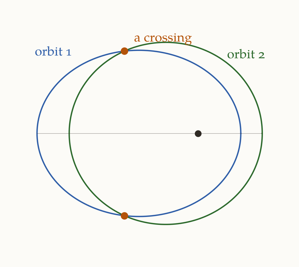
Figure 10 shows such a pair of orbits with a shared apse line. Since the apse line is shared, a point has the same true anomaly \(f\) on both orbits. So the orbits cross where their radii are equal at the same \(f\).
\[ \frac{p_1}{1+e_1\cos f}=\frac{p_2}{1+e_2\cos f}. \]
Cross-multiplying gives \(p_1(1+e_2\cos f)=p_2(1+e_1\cos f)\), and collecting the terms in \(\cos f\) gives
\[ \boxed{\;\cos f^{*}=\frac{p_2-p_1}{p_1e_2-p_2e_1}.\;} \]
The orbits really cross only if \(|\cos f^{*}|\le1\). There are then two crossings, at \(f=\pm f^{*}\). They are mirror images in the apse line, where the radial velocities change sign and the transverse velocities stay the same. The impulse therefore has the same size at both crossings.
Example. Orbit 1 has \(r_p=8000\) km and \(r_a=30\,000\) km. Orbit 2 has \(r_p=12\,000\) km and \(r_a=24\,000\) km. Their apsides are aligned, and \(\mu=398\,600.4418\) km\(^3\)/s\(^2\). Find where they cross and the size of a single impulse there. Then find the cost and the time of the two tangential routes, from periapsis of 1 to apoapsis of 2 and from apoapsis of 1 to periapsis of 2. Which way should we go?
Solution. From the radii, orbit 1 has \(a_1=19\,000\) km, \(e_1=0.578947\) and \(p_1=12\,631.58\) km. Orbit 2 has \(a_2=18\,000\) km, \(e_2=1/3\) and \(p_2=16\,000\) km. The crossing is at
\[ \cos f^{*}=\frac{16\,000-12\,631.58}{12\,631.58\,(0.333333)-16\,000\,(0.578947)}=\frac{3368.42}{-5052.63}=-0.666667 , \]
so \(f^{*}=\pm131.81^\circ\) and \(r^{*}=p_1/(1+e_1\cos f^{*})=20\,571.43\) km. We take the velocity components from \(v_r=(\mu/h)e\sin f\) and \(v_\theta=h/r\), where \(h=\sqrt{\mu p}\). At \(f=+131.81^\circ\), with speeds in km/s,
| \(v_r\) | \(v_\theta\) | \(v\) | Flight path angle \(\gamma\) | |
|---|---|---|---|---|
| Orbit 1 | \(2.42406\) | \(3.44932\) | \(4.21590\) | \(35.098^\circ\) |
| Orbit 2 | \(1.24008\) | \(3.88208\) | \(4.07533\) | \(17.715^\circ\) |
The single impulse is therefore
\[ \Delta v=\sqrt{(1.24008-2.42406)^2+(3.88208-3.44932)^2}=1.26058\text{ km/s}. \]
The two tangential routes are worked out in the same way as before.
| \(a_t\) (km) | \(\Delta v_1\) (km/s) | \(\Delta v_2\) (km/s) | Total (km/s) | Time (h) | |
|---|---|---|---|---|---|
| \(8000\to24\,000\) km | \(16\,000\) | \(0.22459\) | \(0.44580\) | \(0.67039\) | \(2.797\) |
| \(30\,000\to12\,000\) km | \(21\,000\) | \(0.39018\) | \(0.23358\) | \(0.62376\) | \(4.206\) |
The cheaper tangential route costs \(0.624\) km/s. The single impulse costs \(1.26058/0.62376=2.02\) times as much. So we should use the two tangential burns, unless time is very short.
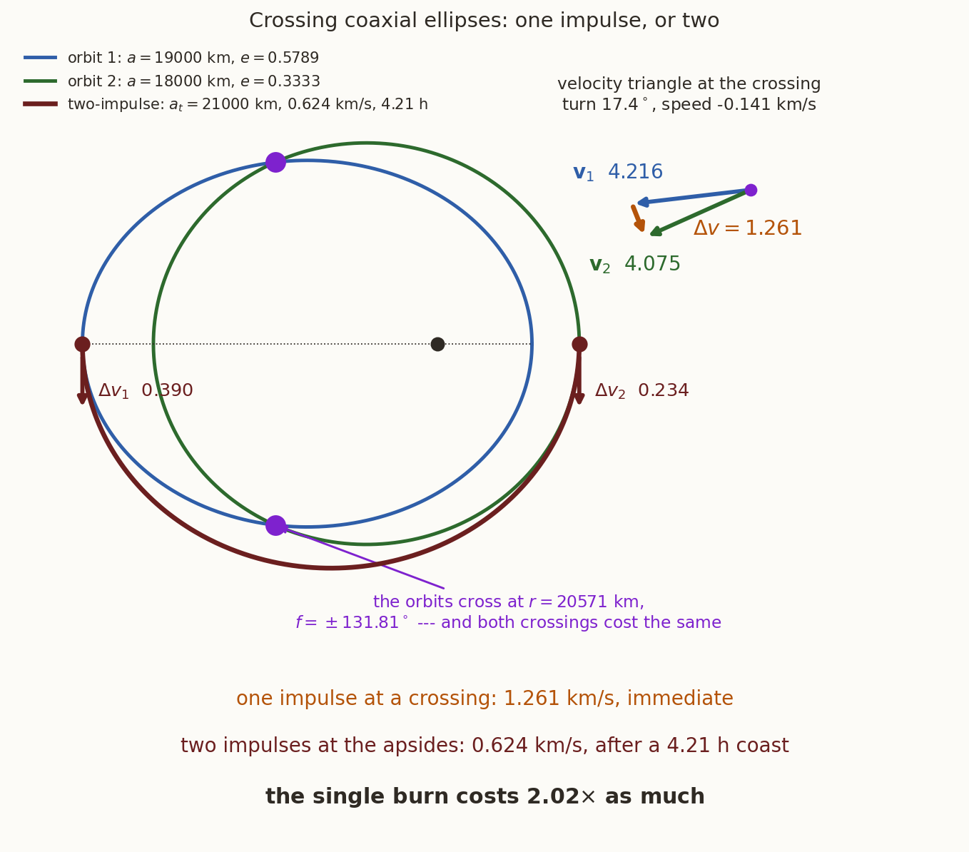
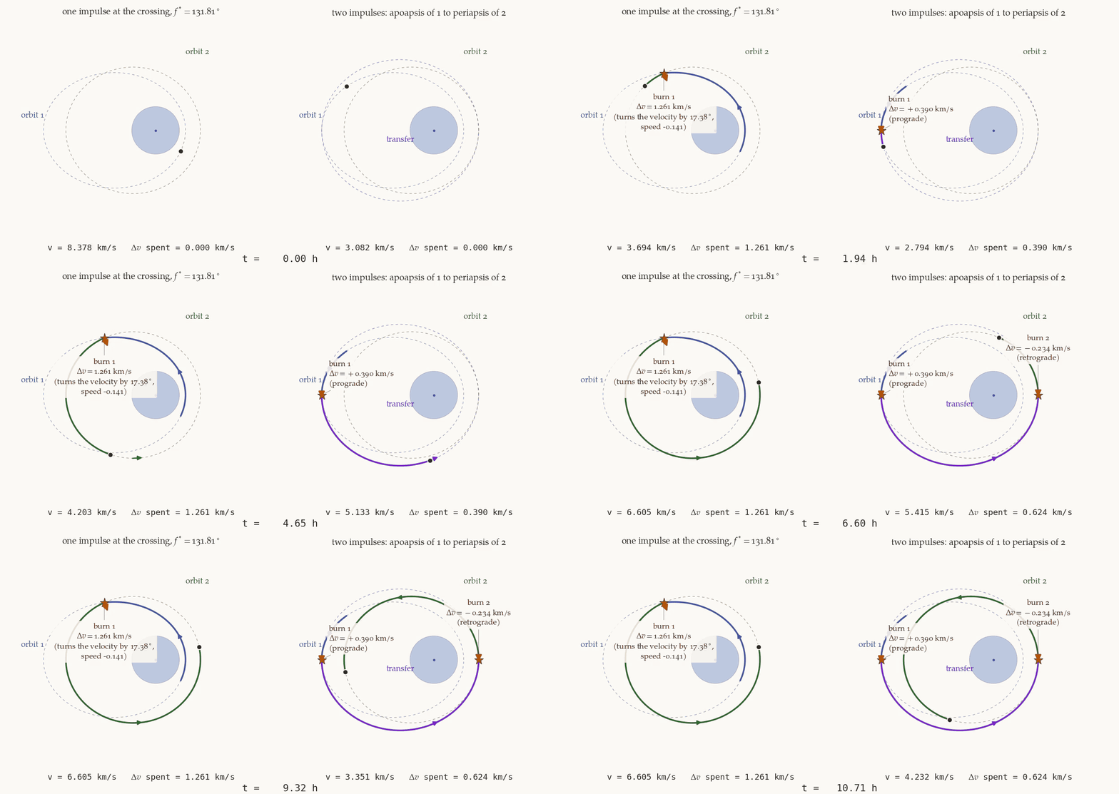
Why is the single impulse so expensive? At the crossing the two speeds are nearly equal, \(4.216\) km/s and \(4.075\) km/s, so very little of the cost goes into changing the speed. Almost all of it goes into turning the velocity, through \(\gamma_1-\gamma_2=17.38^\circ\). Turning a velocity of size \(\bar v\) through an angle \(\theta\) without changing the speed makes an isosceles triangle, whose third side is \(2\bar v\sin(\theta/2)\). At the mean speed \(\bar v=4.146\) km/s this gives \(1.253\) km/s, which is \(99\%\) of the exact cost. So the single burn is really an in-plane version of a plane change. The two-impulse route is cheaper because both of its burns change the size of \(\mathbf v\) and not its direction.
Does the single burn at least save time? It does, but the saving depends on where the spacecraft is when the decision is made. The single burn has to wait for the next crossing. The two-burn route has to wait for the apoapsis of orbit 1 and then coast for \(4.206\) h. Orbit 1 has a period of \(7.240\) h, and Kepler’s equation shows that the crossings are \(2.305\) h from its apoapsis. There are three cases.
| The spacecraft starts | Time saved by the single burn (h) |
|---|---|
| between a crossing and the apoapsis that follows it | \(4.206-2.305=1.90\) |
| between the two crossings, through periapsis | \(2.305+4.206=6.51\) |
| between the apoapsis and the crossing that follows it | \(7.240-2.305+4.206=9.14\) |
So the single burn saves between about \(2\) h and \(9\) h, and the price is large. With \(I_{sp}=320\) s it leaves \(66.9\%\) of the mass, and the two burns leave \(82.0\%\). So a single impulse makes sense only when those hours really matter.
1.5 Why Hohmann is optimal
We chose the Hohmann ellipse because it makes both burns tangential. But a non-tangential burn might still lead to a cheaper transfer overall, because it would allow a different transfer orbit. We now show that this never happens.
The proof has three steps.
- We write both impulses exactly in terms of two properties of the transfer orbit, its energy \(\varepsilon\) and its angular momentum \(h\).
- We show that in these variables the cost increases with \(\varepsilon\) and decreases with \(h\).
- The transfer orbit has to reach both radii, and this restricts the possible values of \((\varepsilon,h)\). We show that the boundary of the allowed region has one corner, and that this corner is the Hohmann ellipse.
Step 1. The impulses in terms of \((\varepsilon,h)\). At radius \(r_i\) the circular velocity has radial component \(0\) and transverse component \(\sqrt{\mu/r_i}\). The transfer orbit has some radial speed \(v_r\) and some transverse speed \(v_\perp=h/r_i\) there. The impulse is the difference of these two velocities, so
\[ \Delta v_i^2=v_r^2+\left(v_\perp-\sqrt{\frac{\mu}{r_i}}\right)^2 =\underbrace{v_r^2+v_\perp^2}_{v^2}-2v_\perp\sqrt{\frac{\mu}{r_i}}+\frac{\mu}{r_i}. \]
The radial speed has disappeared into \(v^2\), and energy gives us \(v^2\), because \(v^2=2(\varepsilon+\mu/r_i)\). We also have \(v_\perp\sqrt{\mu/r_i}=h\sqrt\mu/r_i^{3/2}\). Substituting both,
\[ \boxed{\;\Delta v_i^2=2\varepsilon+\frac{3\mu}{r_i}-\frac{2h\sqrt\mu}{r_i^{3/2}},\qquad i=1,2.\;} \tag{4}\]
This is exact, and we have not assumed that the burn is tangential.
Step 2. How the cost varies. In Equation 4 the coefficient of \(\varepsilon\) is \(+2\), and the coefficient of \(h\) is \(-2\sqrt\mu/r_i^{3/2}\). So both impulses grow with \(\varepsilon\) and shrink with \(h\). The total cost therefore falls as \(h\) grows and as \(\varepsilon\) falls.
Step 3. Which orbits are possible. The transfer orbit has to reach both radii. So its radial speed must be real at both, which needs \(v_r^2=2(\varepsilon+\mu/r_i)-h^2/r_i^2\ge0\). Rearranging,
\[ \varepsilon\ge F(r_i)\equiv\frac{h^2}{2r_i^2}-\frac{\mu}{r_i},\qquad i=1,2 . \]
The cost increases with \(\varepsilon\), so for a given \(h\) the best choice is the smallest allowed \(\varepsilon\), which is the larger of \(F(r_1)\) and \(F(r_2)\). To see which one is larger, we compare them.
\[ F(r_2)-F(r_1)=\left(\frac1{r_2}-\frac1{r_1}\right)\left[\frac{h^2}{2}\left(\frac1{r_1}+\frac1{r_2}\right)-\mu\right]. \]
The first bracket is negative. So \(F(r_2)>F(r_1)\) exactly when the second bracket is negative, which means \(h^2<h_{\rm H}^2\), where
\[ h_{\rm H}^2\equiv\frac{2\mu r_1r_2}{r_1+r_2} . \]
This \(h_{\rm H}\) is the angular momentum of the Hohmann ellipse. The boundary of the allowed region is therefore made of two parabolic arcs that meet at \(h=h_{\rm H}\), and that meeting point is the one corner. There are two cases to consider, one on each side of the corner.
The case \(h\le h_{\rm H}\). Here \(\varepsilon=F(r_2)\), so \(v_r=0\) at \(r_2\). The second burn is tangential, and \(\Delta v_2=\sqrt{\mu/r_2}-h/r_2\), which falls as \(h\) grows. For the first burn, Equation 4 with \(\varepsilon=F(r_2)\) gives \(d\Delta v_1/dh=\left(h/r_2^2-\sqrt\mu/r_1^{3/2}\right)/\Delta v_1\). Since \(h\le h_{\rm H}\),
\[ \frac{h}{r_2^2}\le\frac{\sqrt\mu}{r_2^{3/2}}\sqrt{\frac{2r_1}{r_1+r_2}}<\frac{\sqrt\mu}{r_2^{3/2}}<\frac{\sqrt\mu}{r_1^{3/2}}, \]
so \(\Delta v_1\) also falls as \(h\) grows. The total is smallest at the largest allowed \(h\), which is \(h=h_{\rm H}\).
The case \(h>h_{\rm H}\). Here \(\varepsilon=F(r_1)\), so the first burn is tangential and \(\Delta v_1=h/r_1-\sqrt{\mu/r_1}\), which grows with \(h\). A similar inequality shows that \(\Delta v_2\) grows too. The total is smallest at the smallest allowed \(h\), which is again \(h=h_{\rm H}\).
Both cases lead to \(h=h_{\rm H}\). There the transfer orbit has periapsis \(r_1\), apoapsis \(r_2\) and two tangential burns. This is the Hohmann ellipse, and it is the unique minimum. \(\blacksquare\)
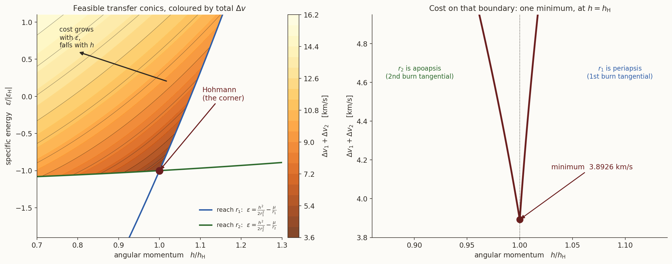
Figure 13 shows the proof as a picture. On the left, every allowed transfer is a point above both parabolas. The cost falls towards the right and downwards, so the cheapest allowed point is the corner. On the right is the cost along the boundary, for the transfer from \(300\) km altitude to the geostationary orbit. It has a sharp minimum at the Hohmann value, \(3.8926\) km/s.
The proof did not assume tangential burns. Where did tangency come from?
Answer
It came from the constraint that the orbit must reach each radius. The cost wants large \(h\) and small \(\varepsilon\), and this constraint stops \(\varepsilon\) from being too small for a given \(h\). Along the boundary \(v_r=0\) at one radius, so the burn there is tangential. At the corner both constraints hold with equality, so both burns are tangential.We should be careful about what the theorem says. It is about two impulses, and it is about \(\Delta v\) alone. It does not rule out a cheaper transfer with more impulses, and the bi-elliptic note shows that three impulses can sometimes do better. It also does not say that Hohmann is the right choice for every mission. It takes half a period of the transfer ellipse, so a mission in a hurry will pay for a faster route.
2 Summary and exercises
The Hohmann transfer (Equation 1) is the cheapest two-impulse transfer between two coplanar circles, for every radius ratio. Its cost is greatest at \(R=15.58\), and beyond this a farther target costs less. Between coaxial ellipses there are always two apsidal routes. With aligned apsides, the route from the periapsis of the inner orbit to the apoapsis of the outer orbit is always the cheaper. Crossing orbits allow a single impulse, but this costs about as much as turning the velocity, and it is usually far more expensive than two tangential burns.
- Going down. A satellite in the geostationary orbit, \(r=42\,164\) km, is to be brought down onto an ellipse whose perigee is at \(100\) km altitude. What single burn does it need, and where? Compare this with the cost of raising it \(300\) km into a graveyard orbit using a Hohmann transfer. Take \(\mu=398\,600.4418\) km\(^3\)/s\(^2\) and \(R_\oplus=6378.137\) km. (Answers: \(1.488\) km/s retrograde, anywhere on the circle. The graveyard orbit costs \(10.9\) m/s in two burns, about \(1/137\) as much. This is why satellites at the end of their lives are raised and not brought down.)
- Proof practice. In the Hohmann optimality proof, carry out the “similar inequality” of the case \(h>h_{\rm H}\) in full. (Hint: write \(d\Delta v_2/dh\) with \(\varepsilon=F(r_1)\), and use \(h>h_{\rm H}\) to bound \(h/r_1^2\) from below.)
All the numbers in this note are checked by hohmann-transfer-verify.py.