The \(f\) and \(g\) Series
Where we are going
The question of the universal-variables note was:
A spacecraft is at position \(\mathbf r_0\) with velocity \(\mathbf v_0\) at time \(t_0\). Where is it a time \(\tau\) later?
Its answer is exact and works for any \(\tau\), but it needs an iteration (the universal Kepler equation) before anything else can be computed. When \(\tau\) is short, a small fraction of an orbit, there is a cheaper answer: the Lagrange coefficients \(F\) and \(G\) can be written as explicit polynomials in \(\tau\), with coefficients computed directly from \(\mathbf r_0\) and \(\mathbf v_0\). No Kepler equation, no orbital elements, and no test of which conic we are on. These polynomials are the \(f\) and \(g\) series, and they are the first step of Gauss’s method of orbit determination (the orbit-determination note), where the state is not yet known and an iteration is impossible.
Names. Textbooks write the Lagrange coefficients \(f\) and \(g\), hence “the \(f\) and \(g\) series”. In these notes \(f\) is the true anomaly, so we write \(F\) and \(G\), as the universal-variables and Lambert notes do. The letters \(u,p,q\) below are those of the orbit-determination texts (Bate, Mueller, and White 1971; Escobal 1965).
The plan:
- Section 1 expands \(\mathbf r(t_0+\tau)\) in a Taylor series and shows that every derivative of \(\mathbf r\) is a combination of \(\mathbf r\) and \(\mathbf v\). This gives a recurrence for the coefficients.
- Section 2 introduces three scalars \(u,p,q\) whose time derivatives are again functions of \(u,p,q\), so that the recurrence becomes pure algebra.
- Section 3 turns the crank up to \(n=5\) and assembles the series, with the velocity series.
- Section 4 checks the result on a circular orbit and against conservation of angular momentum.
- Section 5 measures how good the truncated series is, with a worked example and an interactive figure.
The same material is also available as a slide deck, with animated derivations.
| Symbol | Meaning |
|---|---|
| \(\mathbf r_0,\ \mathbf v_0\) | position and velocity at \(t_0\) |
| \(\tau=t-t_0\) | the time step |
| \(F,\ G,\ \dot F,\ \dot G\) | Lagrange coefficients, \(\mathbf r=F\mathbf r_0+G\mathbf v_0\), \(\mathbf v=\dot F\mathbf r_0+\dot G\mathbf v_0\) |
| \(\mathbf r^{(n)}\) | the \(n\)-th time derivative of \(\mathbf r\) (\(\mathbf r^{(0)}=\mathbf r\), \(\mathbf r^{(1)}=\mathbf v\)) |
| \(F_n,\ G_n\) | scalar coefficients of \(\mathbf r^{(n)}=F_n\mathbf r+G_n\mathbf v\) (Equation 3) |
| \(u=\mu/r^3\) | “local mean motion squared”; \(n^2\) on a circle |
| \(p=\mathbf r\cdot\mathbf v/r^2=\dot r/r\) | relative rate of change of \(r\); not the semi-latus rectum here |
| \(q=v^2/r^2-u\) | departure of the speed from circular speed |
Throughout, \(\mu=398\,600.4418\ \mathrm{km^3/s^2}\) (the Earth). Symbols shared by all the notes are on the notation page.
1 A Taylor series, and a bookkeeping device
1.1 The series
Expand the position about \(t_0\):
\[ \mathbf r(t_0+\tau)=\mathbf r_0+\tau\,\dot{\mathbf r}_0+\frac{\tau^2}{2!}\ddot{\mathbf r}_0+\frac{\tau^3}{3!}\dddot{\mathbf r}_0+\cdots =\sum_{n=0}^{\infty}\frac{\tau^n}{n!}\,\mathbf r^{(n)}_0 . \tag{1}\]
Here the subscript \(0\) means “evaluated at \(t_0\)”. The first two derivatives are given. The second comes from the equation of motion,
\[ \ddot{\mathbf r}=-\frac{\mu}{r^3}\,\mathbf r=-u\,\mathbf r ,\qquad u=\frac{\mu}{r^3}. \tag{2}\]
The third and higher come from differentiating Equation 2 again and again. Done naively, this quickly becomes unmanageable: \(\dddot{\mathbf r}=-\dot u\,\mathbf r-u\,\mathbf v\) needs \(\dot u\), the fourth derivative needs \(\ddot u\), and so on. We need a way to organise the work.
1.2 Every derivative is a combination of \(\mathbf r\) and \(\mathbf v\)
Look at the first few derivatives:
\[ \mathbf r^{(0)}=1\cdot\mathbf r+0\cdot\mathbf v,\qquad \mathbf r^{(1)}=0\cdot\mathbf r+1\cdot\mathbf v,\qquad \mathbf r^{(2)}=-u\,\mathbf r+0\cdot\mathbf v,\qquad \mathbf r^{(3)}=-\dot u\,\mathbf r-u\,\mathbf v . \]
Each is a combination of the current \(\mathbf r\) and \(\mathbf v\) with scalar coefficients \(F_n(t)\), \(G_n(t)\). This is true for every \(n\):
\[ \boxed{\;\mathbf r^{(n)}=F_n\,\mathbf r+G_n\,\mathbf v\;} \tag{3}\]
The geometric reason is that two-body motion stays in the plane spanned by \(\mathbf r\) and \(\mathbf v\), so every derivative of \(\mathbf r\) lies in that plane too, and \(\mathbf r\), \(\mathbf v\) are a basis of it. Figure 1 shows this: whatever the point of the orbit and whatever \(n\), the vector \(\mathbf r^{(n)}\) is the diagonal of a parallelogram built on \(F_n\mathbf r\) and \(G_n\mathbf v\).

1.3 The recurrence
To prove Equation 3, and to compute \(F_n,G_n\), assume it holds for some \(n\) and differentiate once more. Each term is a product of a scalar and a vector, so the product rule gives two terms:
\[ \frac{d}{dt}\bigl(F_n\,\mathbf r\bigr)=\dot F_n\,\mathbf r+F_n\,\dot{\mathbf r}=\dot F_n\,\mathbf r+F_n\,\mathbf v, \qquad \frac{d}{dt}\bigl(G_n\,\mathbf v\bigr)=\dot G_n\,\mathbf v+G_n\,\dot{\mathbf v}. \]
Adding them,
\[ \mathbf r^{(n+1)}=\dot F_n\,\mathbf r+F_n\,\mathbf v+\dot G_n\,\mathbf v+G_n\,\dot{\mathbf v}. \]
The last term contains \(\dot{\mathbf v}\), which is not \(\mathbf r\) or \(\mathbf v\). But the equation of motion Equation 2 says \(\dot{\mathbf v}=-u\,\mathbf r\), so that term points along \(\mathbf r\):
\[ \mathbf r^{(n+1)}=\dot F_n\,\mathbf r+F_n\,\mathbf v+\dot G_n\,\mathbf v-u\,G_n\,\mathbf r . \]
Now collect the terms along \(\mathbf r\) and the terms along \(\mathbf v\):
\[ \mathbf r^{(n+1)}=\bigl(\dot F_n-u\,G_n\bigr)\,\mathbf r+\bigl(F_n+\dot G_n\bigr)\,\mathbf v . \]
This is of the form Equation 3 with \(n+1\) in place of \(n\), which completes the induction (it starts at \(n=0\) with \(F_0=1\), \(G_0=0\)). Reading off the coefficients:
\[ \boxed{\;F_{n+1}=\dot F_n-u\,G_n,\qquad G_{n+1}=F_n+\dot G_n,\qquad F_0=1,\quad G_0=0.\;} \tag{4}\]
1.4 From the recurrence to \(F\) and \(G\)
Evaluate Equation 3 at \(t_0\), where \(\mathbf r=\mathbf r_0\) and \(\mathbf v=\mathbf v_0\), and put it into the Taylor series Equation 1:
\[ \mathbf r(t_0+\tau)=\sum_{n}\frac{\tau^n}{n!}\bigl(F_{n,0}\,\mathbf r_0+G_{n,0}\,\mathbf v_0\bigr). \]
The vectors \(\mathbf r_0\) and \(\mathbf v_0\) are the same in every term, so they can be taken out of the sums:
\[ \mathbf r(t_0+\tau) =\Bigl(\sum_n F_{n,0}\frac{\tau^n}{n!}\Bigr)\mathbf r_0+\Bigl(\sum_n G_{n,0}\frac{\tau^n}{n!}\Bigr)\mathbf v_0 . \]
Comparing with \(\mathbf r=F\mathbf r_0+G\mathbf v_0\) identifies the Lagrange coefficients:
\[ F(\tau)=\sum_{n=0}^{\infty}F_{n,0}\,\frac{\tau^n}{n!},\qquad G(\tau)=\sum_{n=0}^{\infty}G_{n,0}\,\frac{\tau^n}{n!}. \tag{5}\]
Everything vector-valued has been dealt with. What remains is to compute the numbers \(F_{n,0}\) and \(G_{n,0}\). The recurrence needs the time derivatives \(\dot F_n\), \(\dot G_n\), and for that we must know what \(F_n\) and \(G_n\) are functions of.
2 Three scalars that close the system
2.1 The definitions
\[ u=\frac{\mu}{r^3},\qquad p=\frac{\mathbf r\cdot\mathbf v}{r^2}=\frac{\dot r}{r},\qquad q=\frac{v^2}{r^2}-u=\frac{v^2-\mu/r}{r^2}. \tag{6}\]
The second form of \(p\) uses \(r\dot r=\mathbf r\cdot\mathbf v\), which follows from differentiating \(r^2=\mathbf r\cdot\mathbf r\): \(2r\dot r=2\,\mathbf r\cdot\mathbf v\).
What they mean:
- \(u\) has units s\(^{-2}\). On a circular orbit of radius \(r\) the mean motion is \(n=\sqrt{\mu/r^3}\), so \(u=n^2\); in general \(1/\sqrt u\) is the time scale of the motion at the current radius.
- \(p\) has units s\(^{-1}\). It is the relative rate at which the distance changes, and it is zero at periapsis and apoapsis, and everywhere on a circle.
- \(q\) has units s\(^{-2}\). Circular speed at radius \(r\) satisfies \(v^2=\mu/r\), so \(q=0\) when the speed is circular, whatever the direction of the velocity.
Because \(u\tau^2\), \(p\tau\) and \(q\tau^2\) are dimensionless, they are the natural small parameters of a short step.
2.2 Their time derivatives
Three short calculations, each using only \(\dot{\mathbf r}=\mathbf v\), \(\dot{\mathbf v}=-\mu\mathbf r/r^3\) and \(r\dot r=\mathbf r\cdot\mathbf v\).
The derivative of \(u\). By the chain rule,
\[ \dot u=\frac{d}{dt}\bigl(\mu\,r^{-3}\bigr)=-3\mu\,r^{-4}\,\dot r =-3\,\frac{\mu}{r^3}\cdot\frac{\dot r}{r} =-3\,u\,p . \]
The derivative of \(p\). Write \(p=N/D\) with \(N=\mathbf r\cdot\mathbf v\) and \(D=r^2\). Then
\[ \dot N=\mathbf v\cdot\mathbf v+\mathbf r\cdot\dot{\mathbf v}=v^2-\frac{\mu}{r^3}\,\mathbf r\cdot\mathbf r=v^2-\frac{\mu}{r}, \qquad \dot D=2r\dot r=2\,\mathbf r\cdot\mathbf v . \]
By the quotient rule, \(\dot p=\dot N/D-N\dot D/D^2\):
\[ \dot p=\frac{v^2-\mu/r}{r^2}-\frac{(\mathbf r\cdot\mathbf v)\cdot2\,(\mathbf r\cdot\mathbf v)}{r^4} =\Bigl(\frac{v^2}{r^2}-\frac{\mu}{r^3}\Bigr)-2\Bigl(\frac{\mathbf r\cdot\mathbf v}{r^2}\Bigr)^2 =q-2p^2 . \]
The derivative of \(q\). First the speed: \(\dfrac{d}{dt}v^2=2\,\mathbf v\cdot\dot{\mathbf v}=-\dfrac{2\mu}{r^3}\,\mathbf r\cdot\mathbf v\). Then, by the quotient rule,
\[ \frac{d}{dt}\Bigl(\frac{v^2}{r^2}\Bigr) =\frac{1}{r^2}\frac{d v^2}{dt}-\frac{2v^2\dot r}{r^3} =-\frac{2\mu}{r^3}\cdot\frac{\mathbf r\cdot\mathbf v}{r^2}-2\,\frac{v^2}{r^2}\cdot\frac{\dot r}{r} =-2up-2\,(q+u)\,p , \]
where the last step uses \(v^2/r^2=q+u\) from Equation 6. Subtracting \(\dot u=-3up\),
\[ \dot q=-2up-2pq-2pu+3up=-up-2pq=-p\,(u+2q). \]
Collecting the three results:
\[ \boxed{\;\dot u=-3\,u\,p,\qquad \dot p=q-2p^2,\qquad \dot q=-p\,(u+2q).\;} \tag{7}\]
2.3 Why this closes the problem
The right-hand sides of Equation 7 are polynomials in \(u,p,q\). By the product rule, the time derivative of any polynomial in \(u,p,q\) is again a polynomial in \(u,p,q\):
\[ \frac{d}{dt}P(u,p,q)=\frac{\partial P}{\partial u}\,\dot u+\frac{\partial P}{\partial p}\,\dot p+\frac{\partial P}{\partial q}\,\dot q =-3up\,\frac{\partial P}{\partial u}+\bigl(q-2p^2\bigr)\frac{\partial P}{\partial p}-p\,(u+2q)\,\frac{\partial P}{\partial q}. \tag{8}\]
The recurrence Equation 4 starts from the constants \(F_0=1\), \(G_0=0\) and uses only addition, multiplication by \(u\), and time differentiation. So, by induction, every \(F_n\) and \(G_n\) is a polynomial in \(u\), \(p\), \(q\), and Equation 8 differentiates it with no reference to the vectors. The whole computation has become algebra.
3 Turning the crank
3.1 The first coefficients
Apply Equation 4 step by step, differentiating with Equation 8.
\(n=1\). \(F_1=\dot F_0-uG_0=0-0=0\) and \(G_1=F_0+\dot G_0=1+0=1\). So \(\mathbf r^{(1)}=\mathbf v\), as it should be.
\(n=2\). \(F_2=\dot F_1-uG_1=0-u=-u\) and \(G_2=F_1+\dot G_1=0+0=0\). So \(\mathbf r^{(2)}=-u\,\mathbf r\), the equation of motion.
\(n=3\). \(F_3=\dot F_2-uG_2=-\dot u-0=3up\) and \(G_3=F_2+\dot G_2=-u+0=-u\). So
\[ \dddot{\mathbf r}=3up\,\mathbf r-u\,\mathbf v , \]
the jerk. Check it directly: \(\frac{d}{dt}(-u\mathbf r)=-\dot u\,\mathbf r-u\,\mathbf v=3up\,\mathbf r-u\,\mathbf v\).
\(n=4\). For \(F_4\) differentiate \(F_3=3up\) by the product rule, then use Equation 7:
\[ \dot F_3=3\bigl(\dot u\,p+u\,\dot p\bigr)=3\bigl(-3up\cdot p+u\,(q-2p^2)\bigr)=-9up^2+3uq-6up^2=3uq-15up^2 . \]
Then
\[ F_4=\dot F_3-u\,G_3=3uq-15up^2-u\,(-u)=u^2+3uq-15up^2 . \]
For \(G_4\), \(\dot G_3=-\dot u=3up\), so \(G_4=F_3+\dot G_3=3up+3up=6up\).
\(n=5\). Differentiate \(F_4=u^2+3uq-15up^2\) term by term:
\[ \begin{aligned} \frac{d}{dt}\bigl(u^2\bigr)&=2u\,\dot u=-6u^2p,\\ \frac{d}{dt}\bigl(3uq\bigr)&=3\bigl(\dot u\,q+u\,\dot q\bigr)=3\bigl(-3upq-up\,(u+2q)\bigr)=-3u^2p-15upq,\\ \frac{d}{dt}\bigl(-15up^2\bigr)&=-15\bigl(\dot u\,p^2+2up\,\dot p\bigr)=-15\bigl(-3up^3+2up\,(q-2p^2)\bigr)=105up^3-30upq. \end{aligned} \]
Adding, \(\dot F_4=-9u^2p-45upq+105up^3\), and
\[ F_5=\dot F_4-u\,G_4=-9u^2p-45upq+105up^3-6u^2p=15up\,\bigl(7p^2-3q-u\bigr). \]
For \(G_5\): \(\dot G_4=6(\dot u\,p+u\,\dot p)=6\bigl(-3up^2+uq-2up^2\bigr)=6uq-30up^2\), so
\[ G_5=F_4+\dot G_4=u^2+3uq-15up^2+6uq-30up^2=u^2+9uq-45up^2 . \]
| \(n\) | \(F_n\) | \(G_n\) |
|---|---|---|
| \(0\) | \(1\) | \(0\) |
| \(1\) | \(0\) | \(1\) |
| \(2\) | \(-u\) | \(0\) |
| \(3\) | \(3up\) | \(-u\) |
| \(4\) | \(u^2+3uq-15up^2\) | \(6up\) |
| \(5\) | \(15up\,(7p^2-3q-u)\) | \(u^2+9uq-45up^2\) |
| \(6\) | \(-u\,(945p^4-630p^2q-210p^2u+45q^2+24qu+u^2)\) | \(30up\,(14p^2-6q-u)\) |
3.2 The series
Divide each coefficient by \(n!\) and put it into Equation 5. Term by term for \(F\): \(F_2/2!=-u/2\), \(F_3/3!=3up/6=up/2\), \(F_4/4!=\frac{u}{24}(u+3q-15p^2)\), and \(F_5/5!=15up(7p^2-3q-u)/120=\frac{up}{8}(7p^2-3q-u)\). For \(G\): \(G_3/3!=-u/6\), \(G_4/4!=6up/24=up/4\), and \(G_5/5!=\frac{u}{120}(u+9q-45p^2)\). So
\[ \boxed{\; \begin{aligned} F&=1-\frac{u}{2}\tau^2+\frac{up}{2}\tau^3+\frac{u}{24}\bigl(u+3q-15p^2\bigr)\tau^4+\frac{up}{8}\bigl(7p^2-3q-u\bigr)\tau^5+\cdots\\[4pt] G&=\tau-\frac{u}{6}\tau^3+\frac{up}{4}\tau^4+\frac{u}{120}\bigl(u+9q-45p^2\bigr)\tau^5+\cdots \end{aligned}\;} \tag{9}\]
with \(u,p,q\) evaluated at \(t_0\), computed from \(\mathbf r_0\) and \(\mathbf v_0\).
The input is the state and the step, the output is \(\mathbf r=F\mathbf r_0+G\mathbf v_0\). There is no iteration, no element, and no distinction between ellipse, parabola and hyperbola.
3.3 The velocity series
\(\mathbf r_0,\mathbf v_0\) do not depend on \(\tau\), so differentiate \(\mathbf r=F\mathbf r_0+G\mathbf v_0\) term by term, using \(\frac{d}{d\tau}\tau^n=n\tau^{n-1}\) (for example \(\frac{d}{d\tau}\frac{up}{2}\tau^3=\frac{3up}{2}\tau^2\)):
\[ \mathbf v(t_0+\tau)=\frac{dF}{d\tau}\,\mathbf r_0+\frac{dG}{d\tau}\,\mathbf v_0 , \]
\[ \begin{aligned} \dot F&=-u\,\tau+\frac{3up}{2}\tau^2+\frac{u}{6}\bigl(u+3q-15p^2\bigr)\tau^3+\frac{5up}{8}\bigl(7p^2-3q-u\bigr)\tau^4+\cdots\\[4pt] \dot G&=1-\frac{u}{2}\tau^2+up\,\tau^3+\frac{u}{24}\bigl(u+9q-45p^2\bigr)\tau^4+\cdots \end{aligned} \tag{10}\]
Note that \(\dot F\) here means \(dF/d\tau\), with \(u,p,q\) held at their \(t_0\) values. It is not the \(\dot F_n\) of the recurrence, which is a time derivative along the orbit, with \(u,p,q\) changing.
4 Two checks
4.1 The circular orbit
On a circle, \(\dot r=0\) and \(v^2=\mu/r\), so \(p=0\) and \(q=0\), and \(u=n^2\) with \(n\) the mean motion. Set \(p=0\) in Equation 9: the terms \(\frac{up}{2}\tau^3\), \(\frac{up}{8}(\cdots)\tau^5\) of \(F\) and \(\frac{up}{4}\tau^4\) of \(G\) vanish, and the \(\tau^4\) and \(\tau^5\) brackets lose their \(p^2\) parts:
\[ F=1-\frac{u}{2}\tau^2+\frac{u}{24}\,(u+3q)\,\tau^4-\cdots,\qquad G=\tau-\frac{u}{6}\tau^3+\frac{u}{120}\,(u+9q)\,\tau^5-\cdots \]
Now set \(q=0\):
\[ F=1-\frac{u}{2}\tau^2+\frac{u^2}{24}\tau^4-\cdots,\qquad G=\tau-\frac{u}{6}\tau^3+\frac{u^2}{120}\tau^5-\cdots \]
and finally \(u=n^2\), writing \(2=2!\), \(24=4!\), \(6=3!\), \(120=5!\):
\[ F=1-\frac{(n\tau)^2}{2!}+\frac{(n\tau)^4}{4!}-\cdots=\cos n\tau,\qquad G=\tau-\frac{n^2\tau^3}{3!}+\frac{n^4\tau^5}{5!}-\cdots=\frac{\sin n\tau}{n}. \]
So \(\mathbf r=\mathbf r_0\cos n\tau+(\mathbf v_0/n)\sin n\tau\): uniform circular motion. (The verify script checks the agreement through \(\tau^8\).) The odd powers of \(F\) and the even powers of \(G\) all carry a factor \(p\), so \(p\) measures the departure from circular motion: it is what makes the series of an eccentric orbit differ from \(\cos\) and \(\sin\).
4.2 Conservation of angular momentum
Cross \(\mathbf r=F\mathbf r_0+G\mathbf v_0\) with \(\mathbf v=\dot F\mathbf r_0+\dot G\mathbf v_0\). Since \(\mathbf r_0\times\mathbf r_0=\mathbf v_0\times\mathbf v_0=\mathbf 0\) and \(\mathbf v_0\times\mathbf r_0=-\mathbf r_0\times\mathbf v_0\),
\[ \mathbf r\times\mathbf v =F\dot G\,\mathbf r_0\times\mathbf v_0+G\dot F\,\mathbf v_0\times\mathbf r_0 =\bigl(F\dot G-\dot FG\bigr)\,\mathbf r_0\times\mathbf v_0 . \]
The angular momentum is constant, so \(F\dot G-\dot FG=1\) exactly. Check it on the series through \(\tau^3\). Multiply out, keeping powers up to \(\tau^3\):
\[ \begin{aligned} F\dot G&=\Bigl(1-\frac u2\tau^2+\frac{up}2\tau^3\Bigr)\Bigl(1-\frac u2\tau^2+up\,\tau^3\Bigr) =1-\frac u2\tau^2-\frac u2\tau^2+\frac{up}{2}\tau^3+up\,\tau^3+O(\tau^4)\\ &=1-u\tau^2+\frac32up\,\tau^3+O(\tau^4),\\ \dot FG&=\Bigl(-u\tau+\frac32up\,\tau^2\Bigr)\Bigl(\tau-\frac u6\tau^3\Bigr) =-u\tau^2+\frac32up\,\tau^3+O(\tau^4). \end{aligned} \]
The difference is \(1+O(\tau^4)\). A truncated series conserves angular momentum only to its own order; Exercise 3 carries the check one order further.
5 How good is it?
5.1 A worked example
Given. A satellite in low Earth orbit has \(\mathbf r_0=(7000,\ 0,\ 0)\) km and \(\mathbf v_0=(1,\ 7.8,\ 0)\) km/s. Find its position \(\tau=60\) s later from the series through \(\tau^4\), and compare with the exact answer.
Step 1: the three scalars. \(r_0=7000\) km, \(\mathbf r_0\cdot\mathbf v_0=7000\) km\(^2\)/s, \(v_0^2=61.84\) km\(^2\)/s\(^2\), and \(r_0^2=4.9\times10^7\) km\(^2\):
\[ u=\frac{398\,600.4418}{7000^3}=1.162100\times10^{-6}\ \mathrm{s^{-2}},\qquad p=\frac{7000}{4.9\times10^7}=1.428571\times10^{-4}\ \mathrm{s^{-1}}, \]
\[ q=\frac{61.84}{4.9\times10^7}-u=1.262041\times10^{-6}-1.162100\times10^{-6}=9.99404\times10^{-8}\ \mathrm{s^{-2}}. \]
The time scale \(1/\sqrt u=928\) s, so \(\tau=60\) s is short. (For the record, \(a=7659\) km and the period is \(111\) min.)
Step 2: the coefficients. The bracket of the \(\tau^4\) term is \(u+3q-15p^2=1.155799\times10^{-6}\) s\(^{-2}\). With \(\tau=60\) s, term by term,
| \(\tau^0\) or \(\tau^1\) | \(\tau^2\) | \(\tau^3\) | \(\tau^4\) | sum | |
|---|---|---|---|---|---|
| \(F\) | \(1\) | \(-2.091781\times10^{-3}\) | \(1.792955\times10^{-5}\) | \(7.253035\times10^{-7}\) | \(0.997926874\) |
| \(G\) [s] | \(60\) | — | \(-4.183561\times10^{-2}\) | \(5.378865\times10^{-4}\) | \(59.958702272\) |
The terms shrink fast: the \(\tau^2\) term is \(2\times10^{-3}\), and each further power of \(\tau\) brings a factor of order \(\sqrt u\,\tau\approx0.065\) or \(p\tau\approx0.009\).
Step 3: the position. \(\mathbf r=F\mathbf r_0+G\mathbf v_0=(7045.44682,\ 467.67788,\ 0)\) km.
Check. The exact coefficients (universal variables) are \(F=0.997926853\), \(G=59.958710410\) s, giving \((7045.44668,\ 467.67794,\ 0)\) km. The series is off by \(0.15\) m after \(60\) s. The velocity from Equation 10, through \(\tau^3\), is off by \(1.3\) cm/s.
5.2 Over longer steps
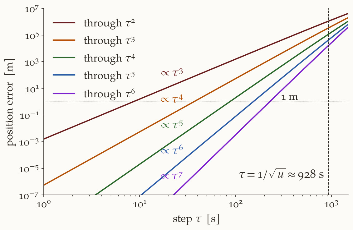
Figure 2 repeats the computation continuously in \(\tau\) and for several truncation orders, and Table 3 lists a few values.
| \(\tau\) | through \(\tau^2\) | through \(\tau^3\) | through \(\tau^4\) | through \(\tau^6\) |
|---|---|---|---|---|
| \(10\) s | \(1.6\) m | \(5.4\) mm | \(0.02\) mm | \(<1\ \mu\)m |
| \(60\) s | \(334\) m | \(6.9\) m | \(0.15\) m | \(0.09\) mm |
| \(300\) s | \(40\) km | \(4.1\) km | \(458\) m | \(6.8\) m |
Two rules can be read off Figure 2:
- Each extra term buys one power of \(\tau\). Truncating after \(\tau^k\) leaves an error proportional to \(\tau^{k+1}\), the straight lines of slope \(k+1\) on the log-log plot.
- The scale is \(1/\sqrt u\) (\(928\) s here, comparable to \(T/2\pi=1061\) s). For \(\tau\ll1/\sqrt u\), a few degrees of arc, the series is excellent. As \(\tau\) approaches \(1/\sqrt u\) all the truncations fail together, and the predicted paths peel away from the true orbit.
The series is therefore a short-step tool. For an eccentric orbit it also has a finite radius of convergence, so adding terms cannot rescue a long step. For long steps use the universal-variable coefficients.
5.3 Where the series is used
In Gauss’s method of angles-only orbit determination the state at the middle observation is unknown, so the exact \(F\) and \(G\) cannot be computed. Keeping only the first two terms of Equation 9,
\[ F\approx1-\frac{u}{2}\tau^2,\qquad G\approx\tau-\frac{u}{6}\tau^3, \]
leaves \(u=\mu/r^3\) as the only unknown, a function of the distance alone. That reduces the method to one polynomial equation in \(r\); the orbit-determination note does this and then replaces the series by the exact coefficients.
History. Gauss’s first approximation in Theoria Motus (1809) is equivalent to keeping these leading terms; the method grew out of his 1801 recovery of Ceres from a short arc (Gauss 1809).
6 Summary
- Two-body motion is planar, so every derivative of \(\mathbf r\) is a combination \(\mathbf r^{(n)}=F_n\mathbf r+G_n\mathbf v\) of the current position and velocity (Equation 3, Figure 1).
- Differentiating once more and using \(\dot{\mathbf v}=-u\mathbf r\) gives the recurrence \(F_{n+1}=\dot F_n-uG_n\), \(G_{n+1}=F_n+\dot G_n\) (Equation 4), and the Taylor series of \(\mathbf r\) becomes \(F\mathbf r_0+G\mathbf v_0\) with \(F=\sum F_{n,0}\tau^n/n!\), \(G=\sum G_{n,0}\tau^n/n!\).
- With \(u=\mu/r^3\), \(p=\mathbf r\cdot\mathbf v/r^2\), \(q=v^2/r^2-u\), the rules \(\dot u=-3up\), \(\dot p=q-2p^2\), \(\dot q=-p(u+2q)\) (Equation 7) make every \(F_n,G_n\) a polynomial in \(u,p,q\).
- The result is the \(f\) and \(g\) series Equation 9 and its derivative Equation 10.
- It reduces to \(\cos n\tau\), \(\sin n\tau/n\) on a circle, and conserves angular momentum to its own order.
- Truncated after \(\tau^k\) its error grows as \(\tau^{k+1}\); it is accurate for \(\tau\ll1/\sqrt u\), and it is the first step of Gauss’s method.
Everything in this note can be reproduced with fg-series-verify.py: the derivative rules from \(\ddot{\mathbf r}=-\mu\mathbf r/r^3\) (sympy), the coefficients to \(n=8\), the circular limit and the angular-momentum identity, and the numbers of Section 5.1 and Table 3 against the exact coefficients of _uv.py.
Exercises
- Directly. Differentiate \(\ddot{\mathbf r}=-u\mathbf r\) twice, using Equation 7, and confirm \(\mathbf r^{(4)}=(u^2+3uq-15up^2)\,\mathbf r+6up\,\mathbf v\).
Solution
Once: \(\dddot{\mathbf r}=-\dot u\,\mathbf r-u\,\mathbf v=3up\,\mathbf r-u\,\mathbf v\). Twice:
\[ \mathbf r^{(4)}=3(\dot u\,p+u\,\dot p)\,\mathbf r+3up\,\mathbf v-\dot u\,\mathbf v-u\,\dot{\mathbf v} =3\bigl(-3up^2+uq-2up^2\bigr)\mathbf r+3up\,\mathbf v+3up\,\mathbf v+u^2\,\mathbf r , \]
which is \((u^2+3uq-15up^2)\,\mathbf r+6up\,\mathbf v\). This is the recurrence done by hand: the term \(-u\dot{\mathbf v}=u^2\mathbf r\) is the \(-uG_3\) of Equation 4.
- The next coefficients. Derive \(F_6\) and \(G_6\) from the recurrence and compare with Table 2.
Hint
\(G_6=F_5+\dot G_5\) is the easier one: \(\dot G_5=2u\dot u+9(\dot u q+u\dot q)-45(\dot u p^2+2up\dot p)\). Expand each product with Equation 7, collect, and add \(F_5\); you should get \(30up(14p^2-6q-u)\). For \(F_6=\dot F_5-uG_5\) write \(F_5=105up^3-45upq-15u^2p\) first.
- Angular momentum, one order further. Keep all four series, Equation 9 and Equation 10, through \(\tau^4\), and show that \(F\dot G-\dot FG=1+O(\tau^5)\).
Solution
Through \(\tau^3\) the check was done in the text. For \(\tau^4\), collect every product of a \(\tau^i\) term and a \(\tau^{4-i}\) term (\(F\) and \(\dot G\) have no \(\tau^1\) term, \(G\) has no \(\tau^2\) term):
\[ F\dot G\Big|_{\tau^4}=\underbrace{\frac u{24}(u+9q-45p^2)}_{1\cdot\dot G_{\tau^4}} +\underbrace{\frac{u^2}{4}}_{(-\frac u2)(-\frac u2)} +\underbrace{\frac u{24}(u+3q-15p^2)}_{F_{\tau^4}\cdot1} =\frac{u^2}{3}+\frac{uq}{2}-\frac{5up^2}{2}, \]
\[ \dot FG\Big|_{\tau^4}=\underbrace{\frac{u^2}{6}}_{(-u)(-\frac u6)} +\underbrace{\frac u6(u+3q-15p^2)}_{\dot F_{\tau^3}\cdot\tau} =\frac{u^2}{3}+\frac{uq}{2}-\frac{5up^2}{2}. \]
They are equal, so the difference has no \(\tau^4\) term. (The verify script checks the identity through \(\tau^7\) with the coefficients to \(n=8\).)
- At periapsis. At periapsis \(p=0\). Write \(F\) and \(G\) through \(\tau^4\) in terms of the periapsis radius \(r_p\), speed \(v_p\) and \(\mu\). Which terms of the circular-orbit series are changed by the eccentricity?
Solution
With \(p=0\): \(F=1-\frac{u}{2}\tau^2+\frac{u}{24}(u+3q)\tau^4\) and \(G=\tau-\frac u6\tau^3\), where \(u=\mu/r_p^3\) and \(q=v_p^2/r_p^2-\mu/r_p^3\). Only the \(\tau^4\) term of \(F\) (and higher terms) feels the eccentricity, through \(q\): at periapsis \(v_p^2>\mu/r_p\), so \(q>0\) and \(F\) decreases more slowly than \(\cos n\tau\) would. The first deviation of the motion from a circle at periapsis is a fourth-order effect.
- How long a step? For the orbit of Section 5.1, how large can \(\tau\) be if a position error of \(1\) m is acceptable and the series is cut after \(\tau^4\)? Check your answer against the figure.
Answer
About \(85\) s. The error through \(\tau^4\) is \(0.15\) m at \(60\) s and grows as \(\tau^5\), so it reaches \(1\) m at \(60\times(1/0.154)^{1/5}\approx87\) s; Figure 2 shows the green curve crossing the \(1\) m line there.
Further reading
The \(f\) and \(g\) series, and its use in orbit determination, are treated in the orbit-determination literature (Escobal 1965; Bate, Mueller, and White 1971; Vallado 2013); the orbit-determination note uses it in Gauss’s method, and the universal-variables note gives the exact coefficients that replace it for long steps.