The \(f\) and \(g\) Series
Propagating a state for a short time, with no Kepler equation
The question
A spacecraft is at \(\mathbf r_0\) with velocity \(\mathbf v_0\) at \(t_0\). Where is it a short time \(\tau\) later?
Two-body motion stays in the plane of \(\mathbf r_0\) and \(\mathbf v_0\), so
\[ \boxed{\;\mathbf r(t_0+\tau)=F(\tau)\,\mathbf r_0+G(\tau)\,\mathbf v_0, \qquad \mathbf v(t_0+\tau)=\dot F(\tau)\,\mathbf r_0+\dot G(\tau)\,\mathbf v_0 .\;} \]
- \(F,G\) are the Lagrange coefficients. Exact formulas exist (in \(\Delta f\), or in the universal anomaly \(\chi\)), but they need Kepler’s equation solved first.
- For a short step we can do better: explicit polynomials in \(\tau\), no iteration, no conic type.
- That is the \(f\) and \(g\) series. It is the workhorse of short-arc orbit determination (Gauss’s method).
Textbooks write \(f,g\). We write \(F,G\) because \(f\) is the true anomaly in this course.
The idea: a Taylor series in time
Expand the position about \(t_0\):
\[ \mathbf r(t_0+\tau)=\mathbf r_0+\tau\,\dot{\mathbf r}_0+\frac{\tau^2}{2!}\ddot{\mathbf r}_0+\frac{\tau^3}{3!}\dddot{\mathbf r}_0+\cdots =\sum_{n=0}^{\infty}\frac{\tau^n}{n!}\,\mathbf r^{(n)}_0 . \qquad(1)\]
What do we know at \(t_0\)?
- \(\mathbf r^{(0)}_0=\mathbf r_0\) and \(\mathbf r^{(1)}_0=\mathbf v_0\): given.
- \(\mathbf r^{(2)}_0=-\dfrac{\mu}{r_0^3}\,\mathbf r_0\): the equation of motion.
- \(\mathbf r^{(3)}_0,\ \mathbf r^{(4)}_0,\dots\): differentiate the equation of motion again and again.
The derivatives get messy fast. We need a bookkeeping device.
The key observation
Every derivative of \(\mathbf r\) is a combination of \(\mathbf r\) and \(\mathbf v\):
\[ \boxed{\;\mathbf r^{(n)}=F_n\,\mathbf r+G_n\,\mathbf v\;} \qquad(2)\]
with scalar coefficients \(F_n(t),\,G_n(t)\).
- True for \(n=0\): \(F_0=1,\ G_0=0\).
- True for \(n=1\): \(F_1=0,\ G_1=1\).
- True for \(n=2\): \(F_2=-\mu/r^3,\ G_2=0\).
- Induction: assume it for \(n\), differentiate once more (next slide).
Geometrically: the motion never leaves the plane spanned by \(\mathbf r\) and \(\mathbf v\), so neither does any derivative.
See it: every derivative lives in the plane
The body runs round the orbit of the later example. The purple arrow is \(\mathbf r^{(n)}\), drawn as the diagonal of the parallelogram on \(F_n\mathbf r\) (maroon) and \(G_n\mathbf v\) (blue). Each \(n\) has its own scale.
The recurrence
Write \(u=\mu/r^3\), so that \(\ddot{\mathbf r}=-u\,\mathbf r\). Start from
\(\displaystyle \mathbf r^{(n)}=\) \(\displaystyle F_n\,\mathbf r\) \(\displaystyle +\;G_n\,\mathbf v\)
and differentiate once, with the product rule on each term.
The recurrence
Write \(u=\mu/r^3\), so that \(\ddot{\mathbf r}=-u\,\mathbf r\). Start from
\(\displaystyle \mathbf r^{(n+1)}=\) \(\displaystyle \dot F_n\,\mathbf r\) \(\displaystyle +\;F_n\,\mathbf v\) \(\displaystyle +\;\dot G_n\,\mathbf v\) \(\displaystyle +\;G_n\,\dot{\mathbf v}\)
\(\dfrac{d}{dt}(F_n\mathbf r)=\dot F_n\mathbf r+F_n\mathbf v\) and \(\dfrac{d}{dt}(G_n\mathbf v)=\dot G_n\mathbf v+G_n\dot{\mathbf v}\).
The recurrence
Write \(u=\mu/r^3\), so that \(\ddot{\mathbf r}=-u\,\mathbf r\). Start from
\(\displaystyle \mathbf r^{(n+1)}=\) \(\displaystyle \dot F_n\,\mathbf r\) \(\displaystyle +\;F_n\,\mathbf v\) \(\displaystyle +\;\dot G_n\,\mathbf v\) \(\displaystyle -\;u\,G_n\,\mathbf r\)
The equation of motion, \(\dot{\mathbf v}=-u\,\mathbf r\): the last term points along \(\mathbf r\).
The recurrence
Write \(u=\mu/r^3\), so that \(\ddot{\mathbf r}=-u\,\mathbf r\). Start from
\(\displaystyle \mathbf r^{(n+1)}=\) \(\displaystyle \dot F_n\,\mathbf r\) \(\displaystyle -\;u\,G_n\,\mathbf r\) \(\displaystyle +\;F_n\,\mathbf v\) \(\displaystyle +\;\dot G_n\,\mathbf v\)
Collect the \(\mathbf r\) terms and the \(\mathbf v\) terms.
The recurrence
Write \(u=\mu/r^3\), so that \(\ddot{\mathbf r}=-u\,\mathbf r\). Start from
\(\displaystyle \mathbf r^{(n+1)}=\) \(\displaystyle \bigl(\dot F_n-u\,G_n\bigr)\,\mathbf r\) \(\displaystyle +\;\bigl(F_n+\dot G_n\bigr)\,\mathbf v\)
Compare with \(\mathbf r^{(n+1)}=F_{n+1}\mathbf r+G_{n+1}\mathbf v\) and read off the coefficients:
\[ \boxed{\;F_{n+1}=\dot F_n-u\,G_n,\qquad G_{n+1}=F_n+\dot G_n,\qquad F_0=1,\quad G_0=0.\;} \qquad(3)\]
To run it we must differentiate \(F_n,G_n\) in time. They will turn out to be functions of three scalars, so we need the time derivatives of those three.
From derivatives to the series
Evaluate at \(t_0\) and substitute into the Taylor series:
\[ \mathbf r(t_0+\tau) =\sum_n\frac{\tau^n}{n!}\bigl(F_{n,0}\,\mathbf r_0+G_{n,0}\,\mathbf v_0\bigr) =\underbrace{\Bigl(\sum_n F_{n,0}\frac{\tau^n}{n!}\Bigr)}_{F(\tau)}\mathbf r_0 +\underbrace{\Bigl(\sum_n G_{n,0}\frac{\tau^n}{n!}\Bigr)}_{G(\tau)}\mathbf v_0 . \]
- The vectors \(\mathbf r_0,\mathbf v_0\) are fixed; only the scalars carry the time dependence.
- \(F_{n,0}\) is \(F_n\) evaluated at \(t_0\): a number once \(\mathbf r_0,\mathbf v_0\) are known.
- So the whole problem reduces to computing the numbers \(F_n,G_n\) at \(t_0\).
Three scalars: \(u\), \(p\), \(q\)
\[ u=\frac{\mu}{r^3},\qquad p=\frac{\mathbf r\cdot\mathbf v}{r^2}=\frac{\dot r}{r},\qquad q=\frac{v^2}{r^2}-u=\frac{v^2-\mu/r}{r^2}. \qquad(4)\]
- \(u\): the “local mean motion squared”. On a circle \(u=n^2\).
- \(p\): the relative rate at which \(r\) changes. It is zero at periapsis and apoapsis.
- \(q\): how far the speed is from circular speed. On a circle \(v^2=\mu/r\), so \(q=0\).
- All three have units of \(\text{time}^{-1}\) or \(\text{time}^{-2}\), so \(u\tau^2\), \(p\tau\), \(q\tau^2\) are the small parameters.
Notation trap
This \(p\) is not the semi-latus rectum. We keep the letters of the orbit-determination texts (Bate, Mueller, and White 1971; Escobal 1965).
Rule 1: \(\dot u=-3\,u\,p\)
\[ u=\mu\,r^{-3} \quad\Longrightarrow\quad \dot u=-3\mu\,r^{-4}\,\dot r=-3\,\frac{\mu}{r^3}\,\frac{\dot r}{r} \]
\[ \boxed{\;\dot u=-3\,u\,p\;} \]
We used \(\dot r=\mathbf r\cdot\mathbf v/r\), which comes from differentiating \(r^2=\mathbf r\cdot\mathbf r\): \(\;2r\dot r=2\,\mathbf r\cdot\mathbf v\).
Rule 2: \(\dot p=q-2p^2\)
\[ p=\frac{\mathbf r\cdot\mathbf v}{r^2} \quad\Longrightarrow\quad \dot p=\frac{\mathbf v\cdot\mathbf v+\mathbf r\cdot\dot{\mathbf v}}{r^2}-\frac{(\mathbf r\cdot\mathbf v)\,2r\dot r}{r^4}. \]
Use \(\dot{\mathbf v}=-\mu\mathbf r/r^3\), so \(\mathbf r\cdot\dot{\mathbf v}=-\mu/r\), and \(r\dot r=\mathbf r\cdot\mathbf v\):
\[ \dot p=\underbrace{\frac{v^2}{r^2}-\frac{\mu}{r^3}}_{q}-2\underbrace{\Bigl(\frac{\mathbf r\cdot\mathbf v}{r^2}\Bigr)^2}_{p^2} \]
\[ \boxed{\;\dot p=q-2p^2\;} \]
Rule 3: \(\dot q=-p\,(u+2q)\)
Speed: \(\dfrac{d}{dt}v^2=2\,\mathbf v\cdot\dot{\mathbf v}=-\dfrac{2\mu}{r^3}\,\mathbf r\cdot\mathbf v\). Then
\[ \frac{d}{dt}\Bigl(\frac{v^2}{r^2}\Bigr) =\frac{-2\mu\,\mathbf r\cdot\mathbf v/r^3}{r^2}-\frac{2v^2\,\dot r}{r^3} =-2up-2\,\frac{v^2}{r^2}\,p =-2up-2p\,(q+u). \]
Subtract \(\dot u=-3up\):
\[ \dot q=-2up-2pq-2pu+3up \qquad\Longrightarrow\qquad \boxed{\;\dot q=-p\,(u+2q)\;} \]
The rules are closed
\[ \boxed{\;\dot u=-3\,u\,p,\qquad \dot p=q-2p^2,\qquad \dot q=-p\,(u+2q).\;} \qquad(5)\]
- The derivative of a polynomial in \(u,p,q\) is again a polynomial in \(u,p,q\).
- The recurrence starts from \(F_0=1,\ G_0=0\) and only adds, multiplies by \(u\) and differentiates.
- So every \(F_n\) and \(G_n\) is a polynomial in \(u,p,q\). The vectors never appear again.
- Differentiating is now pure algebra, which is ideal for a symbolic program (or for a student with patience).
Turning the crank: \(n=1,2,3\)
\(F_{n+1}=\dot F_n-uG_n,\qquad G_{n+1}=F_n+\dot G_n\)
| \(n\) | \(F_n\) | \(G_n\) |
|---|---|---|
| \(0\) | \(1\) | \(0\) |
| \(1\) | \(\dot F_0-uG_0=0\) | \(F_0+\dot G_0=1\) |
| \(2\) | \(\dot F_1-uG_1=-u\) | \(F_1+\dot G_1=0\) |
| \(3\) | \(\dot F_2-uG_2=-\dot u=3up\) | \(F_2+\dot G_2=-u\) |
Each new row is built from the row above it, which lights up in blue.
Check \(n=2\): \(\mathbf r^{(2)}=-u\,\mathbf r\), the equation of motion. ✓
Check \(n=3\): \(\dddot{\mathbf r}=3up\,\mathbf r-u\,\mathbf v\), the jerk. Differentiate \(-u\mathbf r\) directly to confirm.
Turning the crank: \(n=4\)
\[ F_4=\dot F_3-uG_3=\frac{d}{dt}(3up)+u^2=3(\dot u\,p+u\,\dot p)+u^2 \]
\[ =3\bigl(-3up^2+u(q-2p^2)\bigr)+u^2 \qquad\Longrightarrow\qquad \boxed{F_4=u^2+3uq-15up^2} \]
\[ G_4=F_3+\dot G_3=3up-\dot u=3up+3up \qquad\Longrightarrow\qquad \boxed{G_4=6up} \]
The next ones (exercise)
| \(n\) | \(F_n\) | \(G_n\) |
|---|---|---|
| \(4\) | \(u^2+3uq-15up^2\) | \(6up\) |
| \(5\) | \(15up\,(7p^2-3q-u)\) | \(u^2+9uq-45up^2\) |
| \(6\) | \(-u\,(945p^4-630p^2q-210p^2u+45q^2+24qu+u^2)\) | \(30up\,(14p^2-6q-u)\) |
The coefficients grow quickly, and in practice the series is cut off after \(\tau^4\) or \(\tau^5\). These entries, through \(n=8\), are generated and checked by fg-series-verify.py.
The \(f\) and \(g\) series
Divide by \(n!\) and collect powers of \(\tau\):
\[ \boxed{\; \begin{aligned} F&=1-\frac{u}{2}\tau^2+\frac{up}{2}\tau^3+\frac{u}{24}\bigl(u+3q-15p^2\bigr)\tau^4+\frac{up}{8}\bigl(7p^2-3q-u\bigr)\tau^5+\cdots\\[4pt] G&=\tau-\frac{u}{6}\tau^3+\frac{up}{4}\tau^4+\frac{u}{120}\bigl(u+9q-45p^2\bigr)\tau^5+\cdots \end{aligned}\;} \qquad(6)\]
with \(u,p,q\) evaluated at \(t_0\).
Input: \(\mathbf r_0,\mathbf v_0\) and \(\tau\). Output: \(\mathbf r=F\mathbf r_0+G\mathbf v_0\). No elements, no anomalies, no iteration, and no case split between ellipse, parabola and hyperbola.
The velocity series
\(\mathbf r_0,\mathbf v_0\) do not depend on \(\tau\), so differentiate \(\mathbf r=F\mathbf r_0+G\mathbf v_0\) term by term:
\[ \mathbf v(t_0+\tau)=\frac{dF}{d\tau}\,\mathbf r_0+\frac{dG}{d\tau}\,\mathbf v_0 , \]
\[ \begin{aligned} \dot F&=-u\,\tau+\frac{3up}{2}\tau^2+\frac{u}{6}\bigl(u+3q-15p^2\bigr)\tau^3+\frac{5up}{8}\bigl(7p^2-3q-u\bigr)\tau^4+\cdots\\[4pt] \dot G&=1-\frac{u}{2}\tau^2+up\,\tau^3+\frac{u}{24}\bigl(u+9q-45p^2\bigr)\tau^4+\cdots \end{aligned} \qquad(7)\]
Note that \(\dot F\) here means \(dF/d\tau\), with \(u,p,q\) held at their \(t_0\) values. It is not the \(\dot F_n\) of the recurrence, which is a time derivative along the orbit.
Check 1: the circular orbit
On a circle \(\dot r=0\) and \(v^2=\mu/r\), so \(p=0\), \(q=0\), \(u=n^2\):
\(\displaystyle F=\) \(\displaystyle 1\) \(\displaystyle -\frac{u}{2}\tau^2\) \(\displaystyle +\frac{up}{2}\tau^3\) \(\displaystyle +\frac{u}{24}\bigl(u+3q-15p^2\bigr)\tau^4\) \(\displaystyle +\frac{up}{8}\bigl(\cdots\bigr)\tau^5\) \(\displaystyle +\cdots\)
\(\displaystyle G=\) \(\displaystyle \tau\) \(\displaystyle -\frac{u}{6}\tau^3\) \(\displaystyle +\frac{up}{4}\tau^4\) \(\displaystyle +\frac{u}{120}\bigl(u+9q-45p^2\bigr)\tau^5\) \(\displaystyle +\cdots\)
The amber terms carry a factor \(p\).
Check 1: the circular orbit
On a circle \(\dot r=0\) and \(v^2=\mu/r\), so \(p=0\), \(q=0\), \(u=n^2\):
\(\displaystyle F=\) \(\displaystyle 1\) \(\displaystyle -\frac{u}{2}\tau^2\) \(\displaystyle +\frac{up}{2}\tau^3\) \(\displaystyle +\frac{u}{24}\bigl(u+3q-15p^2\bigr)\tau^4\) \(\displaystyle +\frac{up}{8}\bigl(\cdots\bigr)\tau^5\) \(\displaystyle +\cdots\)
\(\displaystyle G=\) \(\displaystyle \tau\) \(\displaystyle -\frac{u}{6}\tau^3\) \(\displaystyle +\frac{up}{4}\tau^4\) \(\displaystyle +\frac{u}{120}\bigl(u+9q-45p^2\bigr)\tau^5\) \(\displaystyle +\cdots\)
\(p=0\): they vanish.
Check 1: the circular orbit
On a circle \(\dot r=0\) and \(v^2=\mu/r\), so \(p=0\), \(q=0\), \(u=n^2\):
\(\displaystyle F=\) \(\displaystyle 1\) \(\displaystyle -\frac{u}{2}\tau^2\) \(\displaystyle +\frac{u^2}{24}\tau^4\) \(\displaystyle +\cdots\)
\(\displaystyle G=\) \(\displaystyle \tau\) \(\displaystyle -\frac{u}{6}\tau^3\) \(\displaystyle +\frac{u^2}{120}\tau^5\) \(\displaystyle +\cdots\)
\(q=0\) as well.
Check 1: the circular orbit
On a circle \(\dot r=0\) and \(v^2=\mu/r\), so \(p=0\), \(q=0\), \(u=n^2\):
\(\displaystyle F=\) \(\displaystyle 1\) \(\displaystyle -\frac{(n\tau)^2}{2!}\) \(\displaystyle +\frac{(n\tau)^4}{4!}\) \(\displaystyle -\cdots\) \(\displaystyle =\cos n\tau\)
\(\displaystyle G=\) \(\displaystyle \tau\) \(\displaystyle -\frac{n^2\tau^3}{3!}\) \(\displaystyle +\frac{n^4\tau^5}{5!}\) \(\displaystyle -\cdots\) \(\displaystyle =\frac{\sin n\tau}{n}\)
So \(\mathbf r=\mathbf r_0\cos n\tau+\dfrac{\mathbf v_0}{n}\sin n\tau\): uniform circular motion. ✓
The odd powers of \(F\) and the even powers of \(G\) (all proportional to \(p\)) vanish. \(p\) measures the eccentric part of the motion.
Check 2: angular momentum
\[ \mathbf h=\mathbf r\times\mathbf v=(F\mathbf r_0+G\mathbf v_0)\times(\dot F\mathbf r_0+\dot G\mathbf v_0) =\bigl(F\dot G-\dot F G\bigr)\,\mathbf r_0\times\mathbf v_0 . \]
Since \(\mathbf h\) is constant, \(\;\boxed{F\dot G-\dot FG=1.}\)
Through \(\tau^3\):
\[ \begin{aligned} F\dot G&=\bigl(1-\tfrac u2\tau^2+\tfrac{up}2\tau^3\bigr)\bigl(1-\tfrac u2\tau^2+up\,\tau^3\bigr)=1-u\tau^2+\tfrac32 up\,\tau^3+O(\tau^4)\\ \dot FG&=\bigl(-u\tau+\tfrac32 up\,\tau^2\bigr)\,\tau+O(\tau^4)=-u\tau^2+\tfrac32 up\,\tau^3+O(\tau^4) \end{aligned} \]
Difference: \(1+O(\tau^4)\). ✓ The truncated series preserves \(\mathbf h\) only to its own order.
How good is it?
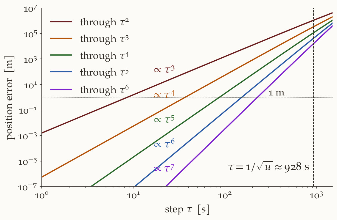
LEO example: \(\mathbf r_0=(7000,0,0)\) km, \(\mathbf v_0=(1,\,7.8,\,0)\) km/s (\(a=7659\) km, \(T=111\) min). Left: the true path (black) and the paths the truncated series predict. Right: their position errors against the exact Lagrange coefficients. Static version: fig-fg-series.png.
How good is it? The numbers
Same example: \(u=1.162\times10^{-6}\ \text{s}^{-2}\), \(p=1.43\times10^{-4}\ \text{s}^{-1}\), \(q=1.0\times10^{-7}\ \text{s}^{-2}\).
| \(\tau\) | through \(\tau^2\) | through \(\tau^3\) | through \(\tau^4\) | through \(\tau^6\) |
|---|---|---|---|---|
| \(10\) s | \(1.6\) m | \(5.4\) mm | \(0.02\) mm | \(<1\ \mu\)m |
| \(60\) s | \(334\) m | \(6.9\) m | \(0.15\) m | \(0.09\) mm |
| \(300\) s | \(40\) km | \(4.1\) km | \(458\) m | \(6.8\) m |
- Truncating after \(\tau^k\) leaves an error \(\propto\tau^{k+1}\): each extra term buys one power of \(\tau\).
- The scale is \(1/\sqrt u\approx 928\) s, comparable to \(T/2\pi\approx1061\) s. The series is excellent for \(\tau\ll1/\sqrt u\), i.e. a few degrees of arc.
- It is not a whole-orbit propagator. For an eccentric orbit the series has a finite radius of convergence. For long steps use the universal-variable \(F,G\).
Where it is used: Gauss’s method
Angles-only orbit determination, with three observations at \(t_1,t_2,t_3\) and \(\tau_i=t_i-t_2\):
\[ \mathbf r_1=F_1\mathbf r_2+G_1\mathbf v_2,\qquad \mathbf r_3=F_3\mathbf r_2+G_3\mathbf v_2 . \]
The state at \(t_2\) is unknown, so the exact \(F,G\) cannot be computed yet. Keep only the first two terms:
\[ F_i\approx1-\frac{u_2}{2}\tau_i^2,\qquad G_i\approx\tau_i-\frac{u_2}{6}\tau_i^3,\qquad u_2=\frac{\mu}{r_2^3}. \]
Only the distance \(r_2\) enters, not the velocity. That is what reduces Gauss’s method to a single polynomial equation in \(r_2\), which is then refined with the exact coefficients. See the orbit-determination notes.
History. Gauss’s first approximation in Theoria Motus (1809) is equivalent to keeping these leading terms. The method grew out of his 1801 recovery of Ceres from a short arc (Gauss 1809).
Summary
- Two-body motion is planar, so every derivative of \(\mathbf r\) is \(F_n\mathbf r+G_n\mathbf v\).
- Differentiating once more gives the recurrence \(F_{n+1}=\dot F_n-uG_n\), \(G_{n+1}=F_n+\dot G_n\).
- With \(u=\mu/r^3\), \(p=\mathbf r\cdot\mathbf v/r^2\), \(q=v^2/r^2-u\), the rules \(\dot u=-3up\), \(\dot p=q-2p^2\), \(\dot q=-p(u+2q)\) make every \(F_n,G_n\) a polynomial in \(u,p,q\).
- Summing the Taylor series gives \(F=1-\tfrac u2\tau^2+\tfrac{up}2\tau^3+\cdots\) and \(G=\tau-\tfrac u6\tau^3+\tfrac{up}4\tau^4+\cdots\).
- Checks: circular orbit (\(\cos n\tau\), \(\sin n\tau/n\)) and \(F\dot G-\dot FG=1\).
- Accurate for \(\tau\ll1/\sqrt u\). It is the first step of Gauss’s method, and the universal-variable \(F,G\) take over for long arcs.
Exercises
- Directly. Differentiate \(\ddot{\mathbf r}=-u\mathbf r\) twice, using the rules for \(\dot u,\dot p,\dot q\), and confirm \(\mathbf r^{(4)}=(u^2+3uq-15up^2)\,\mathbf r+6up\,\mathbf v\).
- The next coefficients. Derive \(F_6\) and \(G_6\) from the recurrence and compare with the table.
- Angular momentum, one order further. Keep all four series through \(\tau^4\), and show that \(F\dot G-\dot FG=1+O(\tau^5)\).
- At periapsis. At periapsis \(p=0\). Write \(F\) and \(G\) through \(\tau^4\) in terms of the periapsis radius \(r_p\), speed \(v_p\) and \(\mu\). Which terms of the circular-orbit series are changed by the eccentricity?
- How long a step? For the orbit of the example, how large can \(\tau\) be if a position error of \(1\) m is acceptable and the series is cut after \(\tau^4\)? Check your answer against the figure.
References

SFM, IIST 2026