Velocity on the Orbit

Devendra Ghate

Where we stand

Solving the two-body problem gave us three constants and one curve:

\[ \mathbf{h} = \mathbf{r}\times\dot{\mathbf{r}}, \qquad \mathbf{e} = \frac{\dot{\mathbf{r}}\times\mathbf{h}}{\mu} - \hat{\mathbf{r}}, \qquad \varepsilon = \frac{v^{2}}{2} - \frac{\mu}{r}, \]

\[ r(f) = \frac{p}{1 + e\cos f}, \qquad p = \frac{h^{2}}{\mu} . \]

The shape is settled. What we do not yet have is the velocity — and every manoeuvre, every \(\Delta v\) budget, every rendezvous is a statement about \(\mathbf{v}\), not about \(r\).

Important

Goal for this deck: given that \(r(f)\) is known, obtain \(\mathbf{v}\) as an explicit function of the true anomaly \(f\) — magnitude and direction — without ever solving for \(t\).

Note that this is possible only because \(f\), not \(t\), is the variable: the hard part of the Kepler problem (inverting \(f(t)\)) never enters.

The two ingredients

We will use exactly two facts, both already proved:

1. The orbit equation. \(r = p/(1 + e\cos f)\), with \(f\) measured from periapsis at the focus.
2. Angular momentum. \(h = r^{2}\dot f = \text{const}\), which is what converts any \(d/df\) into a \(d/dt\):

\[ \frac{d}{dt} = \dot f\,\frac{d}{df} = \frac{h}{r^{2}}\,\frac{d}{df} . \]

That is the whole trick. Differentiation with respect to time costs us nothing, because angular momentum hands us \(\dot f\) for free at every point of the orbit.

Velocity in plane polar coordinates

Work in the orbital plane with the rotating unit vectors \(\hat{\mathbf{r}}\) (radially outward) and \(\hat{\boldsymbol{\theta}}\) (transverse, in the direction of increasing \(f\)). They rotate with the body:

\[ \dot{\hat{\mathbf{r}}} = \dot f\,\hat{\boldsymbol{\theta}}, \qquad \dot{\hat{\boldsymbol{\theta}}} = -\dot f\,\hat{\mathbf{r}} . \]

Differentiating \(\mathbf{r} = r\,\hat{\mathbf{r}}\),

\[ \mathbf{v} = \dot{\mathbf{r}} = \dot r\,\hat{\mathbf{r}} + r\dot f\,\hat{\boldsymbol{\theta}} \;\equiv\; v_r\,\hat{\mathbf{r}} + v_\perp\,\hat{\boldsymbol{\theta}} . \]

So there are only two numbers to find: the radial speed \(v_r = \dot r\) and the transverse speed \(v_\perp = r\dot f\).

Note

\(v_r\) changes the size of \(\mathbf{r}\); \(v_\perp\) changes its direction. Only \(v_\perp\) carries angular momentum — indeed \(h = r v_\perp\).

The transverse component is already known

Angular momentum gives it with no work at all:

\[ v_\perp = r\dot f = \frac{h}{r} = \frac{h}{p}\left(1 + e\cos f\right) . \]

Using \(p = h^{2}/\mu\), the prefactor is \(h/p = \mu/h\):

\[ \boxed{\;v_\perp = \frac{\mu}{h}\left(1 + e\cos f\right)\;} \]

• \(v_\perp > 0\) everywhere the conic exists, since \(1 + e\cos f = p/r > 0\) — the body never reverses its swing.
• \(v_\perp\) is largest at periapsis and smallest at apoapsis, exactly as \(h = rv_\perp = \text{const}\) demands.

The radial component

Differentiate the orbit equation. It is cleanest in reciprocal form:

\[ \frac{1}{r} = \frac{1 + e\cos f}{p} \qquad\Longrightarrow\qquad -\frac{\dot r}{r^{2}} = -\frac{e\sin f}{p}\,\dot f . \]

Hence

\[ \dot r = \frac{r^{2}\dot f}{p}\,e\sin f = \frac{h}{p}\,e\sin f , \]

where \(r^{2}\dot f = h\) was used in the very last step. With \(h/p = \mu/h\) again,

\[ \boxed{\;v_r = \frac{\mu}{h}\,e\sin f\;} \]

Note

Both components carry the same prefactor \(\mu/h = h/p = \sqrt{\mu/p}\). This is the natural speed unit of the orbit — the circular speed at radius \(p\). Every velocity formula below is that number times a pure function of \(e\) and \(f\).

The velocity vector

Putting the two together:

\[ \boxed{\; \mathbf{v}(f) = \frac{\mu}{h}\left[\,e\sin f\;\hat{\mathbf{r}} \;+\;\left(1 + e\cos f\right)\hat{\boldsymbol{\theta}}\,\right] \;} \]

Read off the geometry immediately:

• \(v_r = 0\) at \(f = 0\) and \(f = \pi\) — the apsides are precisely the points where the radius stops growing or shrinking. The velocity there is purely transverse, i.e. perpendicular to \(\mathbf{r}\).
• \(v_r > 0\) on the outbound half \(0 < f < \pi\) and \(v_r < 0\) on the inbound half.
• \(e = 0\) kills \(v_r\) everywhere: circular motion, speed \(\sqrt{\mu/p}\), forever perpendicular to the radius.

The speed

\[ v^{2} = v_r^{2} + v_\perp^{2} = \frac{\mu^{2}}{h^{2}}\left[e^{2}\sin^{2}f + \left(1 + e\cos f\right)^{2}\right] . \]

Expand the bracket:

\[ e^{2}\sin^{2}f + 1 + 2e\cos f + e^{2}\cos^{2}f = 1 + 2e\cos f + e^{2} . \]

So, using \(\mu^2/h^2 = \mu/p\),

\[ \boxed{\;v(f) = \sqrt{\frac{\mu}{p}}\;\sqrt{1 + 2e\cos f + e^{2}}\;} \]

One formula, all four conics. The speed depends on \(f\) only through \(\cos f\), so it is symmetric about the apse line — the body passes any given radius on the way out and on the way in with the same speed, and with flight path angles equal and opposite.

Consistency: this contains vis-viva

Split the bracket deliberately:

\[ 1 + 2e\cos f + e^{2} = \underbrace{2\left(1 + e\cos f\right)}_{= \,2p/r} \;-\;\underbrace{\left(1 - e^{2}\right)}_{=\,p/a} . \]

Therefore

\[ v^{2} = \frac{\mu}{p}\left(\frac{2p}{r} - \frac{p}{a}\right) = \frac{2\mu}{r} - \frac{\mu}{a} , \]

which is the vis-viva equation, and hence \(\varepsilon = -\mu/2a\) once more.

Important

Vis-viva is the magnitude half of what we have just derived. The polar form carries strictly more information: it also fixes the direction of \(\mathbf{v}\), which is what a manoeuvre actually needs.

For the parabola \(e = 1\) the second term vanishes (\(a\to\infty\)) and \(v^{2} = 2\mu/r\) — escape speed at every radius, as it must be.

Flight path angle

Define the flight path angle \(\gamma\) as the angle from the local horizon (the transverse direction) to \(\mathbf{v}\), positive when climbing:

\[ \boxed{\;\tan\gamma = \frac{v_r}{v_\perp} = \frac{e\sin f}{1 + e\cos f}\;} \]

equivalently

\[ \sin\gamma = \frac{e\sin f}{\sqrt{1 + 2e\cos f + e^{2}}},\qquad \cos\gamma = \frac{1 + e\cos f}{\sqrt{1 + 2e\cos f + e^{2}}}, \]

and therefore the frequently used identity

\[ h = r\,v_\perp = r\,v\cos\gamma . \]

\(\gamma\) is the angle by which the velocity is tilted off the local horizontal. \(\gamma = 0\) means the body is momentarily flying “level”.

What \(\gamma\) tells us

• \(\gamma = 0\) at both apsides. A burn at periapsis or apoapsis is purely horizontal — the reason Hohmann transfers are stated there.
• \(\gamma\) has the sign of \(\sin f\): positive outbound, negative inbound.
• Maximum climb. Setting \(d(\tan\gamma)/df = 0\),

\[ \frac{d}{df}\!\left(\frac{e\sin f}{1+e\cos f}\right) = \frac{e\cos f + e^{2}}{\left(1+e\cos f\right)^{2}} = 0 \quad\Longrightarrow\quad \cos f = -e , \]

giving \(\sin\gamma_{\max} = e\), i.e.

\[ \boxed{\;\gamma_{\max} = \arcsin e \quad\text{at}\quad \cos f = -e\;} \]

At that point \(r = p/(1-e^{2}) = a\) and hence \(v = \sqrt{\mu/a}\): the steepest climb happens exactly where the radius equals the semi-major axis, and the speed there is the circular speed for that \(a\).

• For the parabola, \(\tan\gamma = \sin f/(1+\cos f) = \tan(f/2)\), so \(\gamma = f/2\) — an exact, memorable result.

Picture

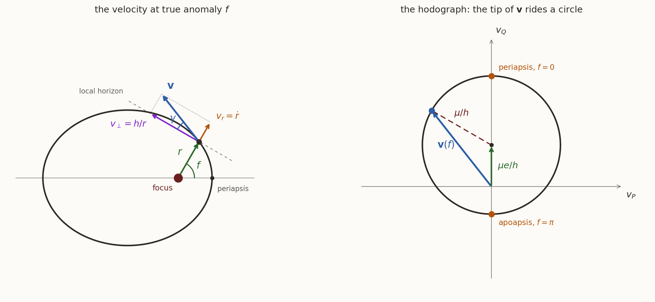
Figure 1: Left: the velocity splits into \(v_r = \dot r = (\mu/h)e\sin f\) along \(\hat{\mathbf{r}}\) and \(v_\perp = h/r = (\mu/h)(1+e\cos f)\) along the local horizon; \(\gamma\) is the tilt of \(\mathbf{v}\) off that horizon. Right: the same velocity plotted in velocity space (perifocal components \(v_P, v_Q\)). As \(f\) runs over the orbit the tip of \(\mathbf{v}\) traces a circle of radius \(\mu/h\) whose centre is displaced \(\mu e/h\) perpendicular to the apse line. The topmost and bottommost points of that circle are periapsis and apoapsis.

The hodograph, derived in one line

The component form hides something remarkable. Go back to the eccentricity-vector integral,

\[ \dot{\mathbf{r}}\times\mathbf{h} = \mu\left(\hat{\mathbf{r}} + \mathbf{e}\right), \]

and cross it with \(\mathbf{h}\) from the left. Using \(\mathbf{h}\times(\mathbf{v}\times\mathbf{h}) = h^{2}\mathbf{v} - \mathbf{h}(\mathbf{h}\cdot\mathbf{v})\) and \(\mathbf{h}\cdot\mathbf{v} = 0\),

\[ \boxed{\;\mathbf{v} = \frac{\mu}{h}\,\hat{\mathbf{h}}\times\left(\hat{\mathbf{r}} + \mathbf{e}\right)\;} \]

Now read it: \(\hat{\mathbf{h}}\times\) is just a \(90^{\circ}\) rotation inside the orbital plane. So \(\mathbf{v}\) is

\[ \underbrace{\frac{\mu}{h}\,\hat{\mathbf{h}}\times\hat{\mathbf{r}}}_{\text{unit vector, rotating with }f} \;+\; \underbrace{\frac{\mu}{h}\,\hat{\mathbf{h}}\times\mathbf{e}}_{\text{fixed vector}} . \]

A vector of constant length \(\mu/h\) sweeping a full turn, added to a constant vector. The tip of \(\mathbf{v}\) therefore moves on a circle of radius \(\mu/h\) centred at distance \(\mu e/h\) from the origin of velocity space, perpendicular to \(\mathbf{e}\). This curve is the hodograph.

The hodograph in components

In the perifocal frame \((\hat{\mathbf{P}}\) towards periapsis, \(\hat{\mathbf{Q}}\) at \(90^{\circ}\) in the direction of motion\()\), substituting \(\hat{\mathbf{r}} = \cos f\,\hat{\mathbf{P}} + \sin f\,\hat{\mathbf{Q}}\):

\[ \boxed{\; v_P = -\frac{\mu}{h}\sin f, \qquad v_Q = \frac{\mu}{h}\left(e + \cos f\right) \;} \]

\[ \Longrightarrow\quad v_P^{2} + \left(v_Q - \frac{\mu e}{h}\right)^{2} = \left(\frac{\mu}{h}\right)^{2} . \]

• Every Kepler orbit — ellipse, parabola or hyperbola — has a circular hodograph. Only the portion traversed differs: the ellipse goes round and round, the hyperbola covers only the arc \(|f| < \arccos(-1/e)\) and the two missing endpoints are the incoming and outgoing \(\mathbf{v}_\infty\).
• \(e < 1\) puts the velocity-space origin inside the circle (every direction of flight is achieved); \(e > 1\) puts it outside (the flight direction is confined to a wedge — the turning angle of a flyby).

Historical note

Hamilton published the circularity of the hodograph in 1846 and used it to give a purely geometric proof of Kepler’s laws; Möbius and Maxwell used it as a teaching device. It is the cleanest statement of “the inverse-square law is special”.

Speed and flight path angle across the conics

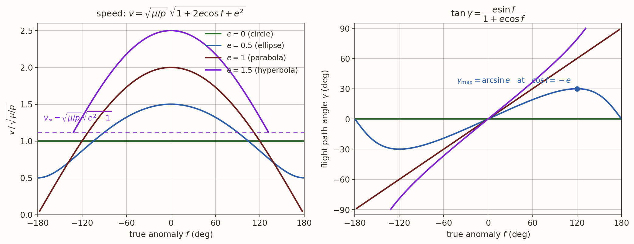
Figure 2: Speed (left) and flight path angle (right) against true anomaly, in units of \(\sqrt{\mu/p}\). Circle: constant speed, \(\gamma \equiv 0\). Ellipse: maximum at periapsis, minimum at apoapsis, \(\gamma\) peaking at \(\arcsin e\) where \(\cos f = -e\). Parabola: speed falls to zero as \(f\to\pm180^{\circ}\) (rest at infinity) and \(\gamma = f/2\) exactly. Hyperbola: the curve stops at the asymptote \(\cos f = -1/e\), where the speed has not decayed to zero but to \(v_\infty = \sqrt{\mu/p}\,\sqrt{e^{2}-1} = \sqrt{\mu/|a|}\).

Apsidal speeds

Put \(f = 0\) and \(f = \pi\) in the boxed speed formula:

\[ v_p = \sqrt{\frac{\mu}{p}}\left(1 + e\right) = \sqrt{\frac{\mu}{a}\,\frac{1+e}{1-e}}, \qquad v_a = \sqrt{\frac{\mu}{p}}\left(1 - e\right) = \sqrt{\frac{\mu}{a}\,\frac{1-e}{1+e}} . \]

Two consequences worth remembering:

\[ \frac{v_p}{v_a} = \frac{1+e}{1-e} = \frac{r_a}{r_p}, \qquad v_p\,v_a = \frac{\mu}{p}\left(1-e^{2}\right) = \frac{\mu}{a} = n^{2}a^{2} . \]

The first is just \(h = rv\) at the apsides (angular momentum). The second says the geometric mean of the apsidal speeds is the circular speed at radius \(a\).

An orbit is raised by a small burn \(\Delta v\) applied horizontally at periapsis. Using \(v_p = \sqrt{\mu/p}\,(1+e)\) and \(h = r_pv_p\), show that \(r_a\) changes far more than \(r_p\) does. Where does the extra energy go?

Limiting cases

Orbit	\(e\)	\(v(f)\)	\(\gamma\)	hodograph
circle	\(0\)	\(\sqrt{\mu/a}\), constant	\(0\)	circle centred at origin
ellipse	\(0<e<1\)	\(\sqrt{\mu/p}\sqrt{1+2e\cos f + e^{2}}\)	\(\lvert\gamma\rvert\le\arcsin e\)	origin inside
parabola	\(1\)	\(\sqrt{2\mu/r} = 2\sqrt{\mu/p}\,\left|\cos\tfrac f2\right|\)	\(f/2\)	origin on the circle
hyperbola	\(>1\)	as above, \(\to v_\infty\)	\(\to\) asymptote value	origin outside

For the hyperbola, at \(\cos f = -1/e\),

\[ v_\infty^{2} = \frac{\mu}{p}\left(1 - 2 + e^{2}\right) = \frac{\mu}{p}\left(e^{2}-1\right) = \frac{\mu}{|a|} = C_3 , \]

recovering the characteristic energy from the escape-velocity slide.

Worked example — a GTO

A geostationary transfer orbit: perigee altitude \(300\) km, apogee at the geostationary radius. With \(\mu_\oplus = 3.986\times10^{5}\ \mathrm{km^{3}/s^{2}}\),

\[ r_p = 6678\ \mathrm{km},\quad r_a = 42164\ \mathrm{km} \;\Longrightarrow\; a = \frac{r_p + r_a}{2} = 24421\ \mathrm{km},\quad e = \frac{r_a - r_p}{r_a + r_p} = 0.7266 . \]

\[ v_p = \sqrt{\frac{\mu}{a}\frac{1+e}{1-e}} = 10.15\ \mathrm{km/s}, \qquad v_a = 1.608\ \mathrm{km/s}, \qquad \frac{v_p}{v_a} = 6.31 = \frac{r_a}{r_p}\ \checkmark \]

The steepest climb occurs at \(\cos f = -e\), i.e. \(f = 136.6^{\circ}\), where \(\gamma = \arcsin 0.7266 = 46.6^{\circ}\), \(r = a = 24421\) km and \(v = \sqrt{\mu/a} = 4.04\) km/s.

At which true anomaly is the spacecraft moving at exactly the local circular speed \(\sqrt{\mu/r}\)? (Hint: set \(v^{2} = \mu/r\) in vis-viva — the answer is \(r = a\), the same point as \(\gamma_{\max}\). Coincidence?)

Summary

Given \(r(f)\) and \(h\) alone:

\[ v_r = \frac{\mu}{h}e\sin f, \qquad v_\perp = \frac{\mu}{h}\left(1 + e\cos f\right), \qquad v = \sqrt{\frac{\mu}{p}}\sqrt{1 + 2e\cos f + e^{2}} , \]

\[ \tan\gamma = \frac{e\sin f}{1+e\cos f}, \qquad \mathbf{v} = \frac{\mu}{h}\,\hat{\mathbf{h}}\times\left(\hat{\mathbf{r}}+\mathbf{e}\right) . \]

• The speed formula is vis-viva, rewritten in \(f\); the polar form adds direction.
• The apsides are exactly the \(\gamma = 0\) points.
• The hodograph is a circle for every conic — a signature of the inverse-square law.

Next: with \(\mathbf{r}(f)\) and \(\mathbf{v}(f)\) both in hand, the state vector in the perifocal frame is complete, and only a rotation stands between us and \(\mathbf{r},\mathbf{v}\) in the inertial frame.