Two body Problem
From earlier equations (from the N-body Problem), we have
\[
\ddot{\mathbf{R}}_2 - \ddot{\mathbf{R}}_1 = \frac{G m_1}{r_{21}^{3}} \mathbf{r}_{21} - \frac{G m_2}{r_{12}^{3}} \mathbf{r}_{12} = -G (m_1 + m_2)\,\frac{\mathbf{r}_{12}}{r_{12}^{3}}
\]
which is clearly,
\[
\ddot{\mathbf{r}}_{12} + \frac{G (m_1 + m_2)}{r_{12}^{3}} \mathbf{r}_{12} = 0
\]
Dropping the subscript, we have
\[
\ddot{\mathbf{r}} + \frac{\mu}{r^{3}} \mathbf{r} = 0, \qquad \mu = G (m_1 + m_2)
\]
Here \(\mu\) is called the standard gravitational parameter. It is a measure of the strength of the gravitational field of the two-body system. So to analyse the two-body problem, we don’t need to know the individual masses, but only this constant.
In the early development of celestial mechanics, the standard gravitational parameter was often used instead of the individual masses. Also, since the mass of the Sun is so much larger than the mass of any planet, as long as they had a good estimate of the mass of the Sun, they could calculate the orbits of the planets without knowing their masses.
We need to solve only this nonlinear second order ODE to get the relative motion of the two bodies. The individual motions can be recovered from the relative motion after that. We will see this process in the Example 1.
Angular Momentum Conservation
We will proceed as the previous section, and calculate all the integrals of motion.
Taking a cross product of the equation with \(\mathbf{r}\), we have
\[
\mathbf{r} \times \ddot{\mathbf{r}} = 0
\]
Since, \(\frac{d}{dt}(\mathbf{r} \times \dot{\mathbf{r}}) = \mathbf{r} \times \ddot{\mathbf{r}}\), we have
\[
\frac{d}{dt}(\mathbf{r} \times \dot{\mathbf{r}}) = 0
\]
Defining \(\mathbf{h} = \mathbf{r} \times \dot{\mathbf{r}}\), we have \(\frac{d\mathbf{h}}{dt} = 0\). Therefore, \(\mathbf{h}\) is a constant vector. This will only happen if the motion is planar. Therefore, the relative motion of the two bodies is planar. This only means that \(\mathbf{r}(t)\) remains in a single plane.
This is a strong geometric statement: the trajectory in 3D collapses to a curve in a single 2D plane. From here on, we can do orbital geometry in two dimensions.
Now let us recall Kepler’s second law, which states that the line joining the two bodies sweeps out equal areas in equal times. This is a consequence of the conservation of angular momentum.
Since \(\mathbf{h}\) is constant, the areal velocity is also constant.
Is \(h=0\) possible? If yes, what kind of motion will this result in?
Answer
Yes. \(\mathbf{h} = \mathbf{r}\times\dot{\mathbf{r}} = \mathbf{0}\) exactly when \(\mathbf{r}\) and \(\dot{\mathbf{r}}\) are parallel, so the motion is rectilinear: a straight line through the centre of attraction. Dropping a body from rest is the standard example.
The conic degenerates with it: \(p = h^{2}/\mu = 0\) and \(e = 1\) whatever the energy, so \((a, e)\) stops describing a shape. Energy still sorts the cases — \(\varepsilon < 0\) rises, stops and falls back; \(\varepsilon = 0\) is the rectilinear parabola; \(\varepsilon > 0\) escapes. This is the \(h = 0\) caveat that makes \(e = 1\) ambiguous.
Eccentricity Vector
Let us post multiply the equation of motion with \(\mathbf{h}\) to get
\[
\ddot{\mathbf{r}} \times \mathbf{h} = -\frac{\mu}{r^3} \mathbf{r} \times \mathbf{h} = -\frac{\mu}{r^3} \mathbf{r} \times \mathbf{r} \times \dot{\mathbf{r}}
\]
Since \(\mathbf{a} \times (\mathbf{b} \times \mathbf{c}) = (\mathbf{a} \cdot \mathbf{c})\mathbf{b} - (\mathbf{a} \cdot \mathbf{b})\mathbf{c}\), we have
\[
\ddot{\mathbf{r}} \times \mathbf{h} = -\frac{\mu}{r^3} \left[ (\mathbf{r} \cdot \dot{\mathbf{r}})\mathbf{r} - (\mathbf{r} \cdot \mathbf{r})\dot{\mathbf{r}} \right] = -\frac{\mu}{r^3} \left[ (\mathbf{r} \cdot \dot{\mathbf{r}})\mathbf{r} - r^2\dot{\mathbf{r}} \right]
\]
Since \(\mathbf{r} = r \hat{\mathbf{r}}\), we have \(\dot{\mathbf{r}} = \dot{r} \hat{\mathbf{r}} + r \dot{\hat{\mathbf{r}}}\),
\[
\begin{aligned}
\mathbf{r} \cdot \dot{\mathbf{r}} & = & r \hat{\mathbf{r}} \cdot (\dot{r} \hat{\mathbf{r}} + r \dot{\hat{\mathbf{r}}})\\
& = & r \dot{r} \hat{\mathbf{r}} \cdot \hat{\mathbf{r}} + r^2 \hat{\mathbf{r}} \cdot \dot{\hat{\mathbf{r}}}\\
& = & r \dot{r} + 0\\
\end{aligned}
\]
We have used, \(\frac{d}{dt}(\hat{\mathbf{r}} \cdot \hat{\mathbf{r}}) = 0\), which implies \(\hat{\mathbf{r}} \cdot \dot{\hat{\mathbf{r}}} = 0\).
Therefore,
\[
\ddot{\mathbf{r}} \times \mathbf{h} = -\frac{\mu}{r^3} \left[ r \dot{r} \mathbf{r} - r^2\dot{\mathbf{r}} \right] = \mu \left( \frac{\dot{\mathbf{r}}}{r} - \frac{\dot{r} \mathbf{r}}{r^2} \right)
\]
Since, \[
\frac{d}{dt}\left( \frac{\mathbf{r}}{r} \right) = \frac{\dot{\mathbf{r}}}{r} - \frac{\dot{r}}{r^2}\mathbf{r}
\]
we have,
\[
\ddot{\mathbf{r}} \times \mathbf{h} = \mu \frac{d}{dt}\left( \frac{\mathbf{r}}{r} \right)
\]
Since \(\mathbf{h}\) is constant, integrating both sides gives
\[
\dot{\mathbf{r}} \times \mathbf{h} = \mu \left( \frac{\mathbf{r}}{r} + \mathbf{e} \right)
\]
Here, \(\mathbf{e}\) is a dimensionless constant vector. We note that it is perpendicular to both the \(\mathbf{h}\) and \(\dot{\mathbf{r}}\) vectors. Since \(\mathbf{h}\) is a constant vector, \(\mathbf{e}\) clearly lies in the orbital plane.
Rearranging previous equation we get,
\[
\mathbf{e} = \frac{\dot{\mathbf{r}} \times \mathbf{h}}{\mu} - \frac{\mathbf{r}}{r}
\]
Differentiating with respect to time, and using \(\dot{\mathbf{h}} = 0\),
\[
\dot{\mathbf{e}} = \frac{\ddot{\mathbf{r}} \times \mathbf{h}}{\mu} - \frac{d}{dt}\left( \frac{\mathbf{r}}{r} \right)
\]
But we have already shown that \(\ddot{\mathbf{r}} \times \mathbf{h} = \mu \frac{d}{dt}\left( \frac{\mathbf{r}}{r} \right)\), and hence the two terms cancel exactly,
\[
\dot{\mathbf{e}} = \mathbf{0}
\]
Let us also show that both its magnitude and its direction are fixed.
Magnitude. Writing \(e = |\mathbf{e}|\),
\[
\frac{d}{dt}\left( e^2 \right) = \frac{d}{dt}(\mathbf{e} \cdot \mathbf{e}) = 2\, \mathbf{e} \cdot \dot{\mathbf{e}} = 0
\quad \Longrightarrow \quad e = \text{constant}
\]
Direction. With \(\hat{\mathbf{e}} = \mathbf{e}/e\), and using \(\dot{e} = 0\) from above,
\[
\dot{\hat{\mathbf{e}}} = \frac{\dot{\mathbf{e}}}{e} - \frac{\dot{e}}{e^2}\mathbf{e} = \mathbf{0} - \mathbf{0} = \mathbf{0}
\quad \Longrightarrow \quad \hat{\mathbf{e}} = \text{constant}
\]
So \(\mathbf{e}\) picks out one fixed line in the orbital plane, for all time.
\(\mathbf{h}\) fixes the plane of motion, while \(\mathbf{e}\) additionally fixes an orientation within that plane. We shall soon see that this fixed direction points towards the point of closest approach (the periapsis), and that \(e\) is precisely the eccentricity of the conic. Its constancy is therefore the statement that the orbit does not precess — the ellipse traced out is closed, and returns on itself.
Precession is the change in the direction of the rotational axis of a spinning object.
The vector \(\mu\,\mathbf{e}\) is known as the Laplace–Runge–Lenz vector, and its conservation is special to the inverse-square law. Any perturbation to \(1/r^2\) — oblateness of the central body, a third body, or the corrections of general relativity — makes \(\dot{\mathbf{e}} \neq \mathbf{0}\), and the apsidal line (line passing through the periapsis and apoapsis) then slowly rotates. The residual perihelion precession of Mercury is the most famous instance of exactly this. Under certain conditions, it may change the shape of the orbit itself.
Example 1
![]()
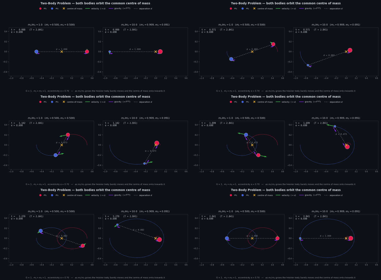
Figure 1: Two-body motion at two mass ratios. Both panels share the same total mass, the same initial separation and the same eccentricity (\(e = 0.70\)); only \(m_1/m_2\) differs. Green arrows are velocities (drawn to scale), purple arrows the gravitational forces (drawn to a compressed \(F^{1/3}\) scale, since \(F \propto 1/d^2\) spans too wide a range). Download the script.
What the animation shows
The centre of mass never moves. Taking the origin at the barycentre, the two bodies stay diametrically opposite about it: \(m_1 \mathbf{R}_1 + m_2
\mathbf{R}_2 = \mathbf{0}\) at every instant.
With \(\mathbf{r} = \mathbf{r}_{12} = \mathbf{R}_2 - \mathbf{R}_1\) and \(M = m_1
+ m_2\) as before, the relative coordinate obeys \(\ddot{\mathbf{r}} =
-GM\,\mathbf{r}/r^3\), and the individual orbits are recovered from \[\mathbf{R}_1 = -\frac{m_2}{M}\,\mathbf{r}, \qquad \mathbf{R}_2 = \frac{m_1}{M}\,\mathbf{r}.\] So each body traces a similar conic about the centre of mass: same shape, same eccentricity, sizes in the inverse ratio of the masses. Note the weights are crossed — body 1 is scaled by \(m_2\) — so the heavier body gets the smaller orbit.
How to find \(R_1\) and \(R_2\)
Define the change of variables \((\mathbf{R}_1, \mathbf{R}_2) \mapsto
(\mathbf{R}_{cm}, \mathbf{r})\):
\[
\begin{aligned}
\mathbf{R}_{cm} &= \frac{m_1}{M}\mathbf{R}_1 + \frac{m_2}{M}\mathbf{R}_2, \\
\mathbf{r} &= -\mathbf{R}_1 + \mathbf{R}_2 .
\end{aligned}
\]
In matrix form, acting componentwise on each Cartesian component,
\[
\begin{pmatrix} \mathbf{R}_{cm} \\ \mathbf{r} \end{pmatrix}
=
\underbrace{\begin{pmatrix} m_1/M & m_2/M \\ -1 & 1 \end{pmatrix}}_{\displaystyle A}
\begin{pmatrix} \mathbf{R}_1 \\ \mathbf{R}_2 \end{pmatrix}.
\]
- It is invertible as \[
\det A = \frac{m_1}{M} + \frac{m_2}{M} = 1 \neq 0 .
\]
Invert \(A\) directly:
\[
A^{-1} = \frac{1}{\det A}\begin{pmatrix} 1 & -m_2/M \\ 1 & \phantom{-}m_1/M\end{pmatrix}
= \begin{pmatrix} 1 & -m_2/M \\ 1 & \phantom{-}m_1/M\end{pmatrix},
\]
that is,
\[
\boxed{\;
\begin{aligned}
\mathbf{R}_1(t) &= \mathbf{R}_{cm}(t) - \frac{m_2}{M}\,\mathbf{r}(t), \\[4pt]
\mathbf{R}_2(t) &= \mathbf{R}_{cm}(t) + \frac{m_1}{M}\,\mathbf{r}(t).
\end{aligned}\;}
\]
The two forces are equal and opposite (Newton’s third law), but the accelerations are not: the heavier body responds \(m_1/m_2\) times less.
Velocities can also be calculated in a similar fashion.
Towards the restricted problem
As \(m_1/m_2\) grows, the orbit of the heavier body shrinks and the centre of mass sinks towards its centre — this is the approximation of the previous section, now visible.
For the Sun-Jupiter pair, \(m_1/m_2 \approx 1047\), so the Sun’s orbit about the barycentre is \(1/1047\) of Jupiter’s. It is small, but not zero: the barycentre lies about \(1.07\) solar radii from the centre of the Sun, i.e. just outside its surface.
This justifies the use of restricted two body problem as a model to predict planetary trajectories.
Example 2
Take \(G = 1\), so that \(\mu = G(m_1 + m_2) = 1\):
\[
\begin{aligned}
m_1 = m_2 &= \tfrac{1}{2}, \\[4pt]
\mathbf{R}_1(0) &= \left(+\tfrac{1}{2},\, 0,\, 0\right), &\qquad
\mathbf{V}_1(0) &= \tfrac{1}{2}\,\hat{\mathbf{y}}, \\
\mathbf{R}_2(0) &= \left(-\tfrac{1}{2},\, 0,\, 0\right), &\qquad
\mathbf{V}_2(0) &= \tfrac{1}{2}\,\hat{\mathbf{z}} .
\end{aligned}
\]
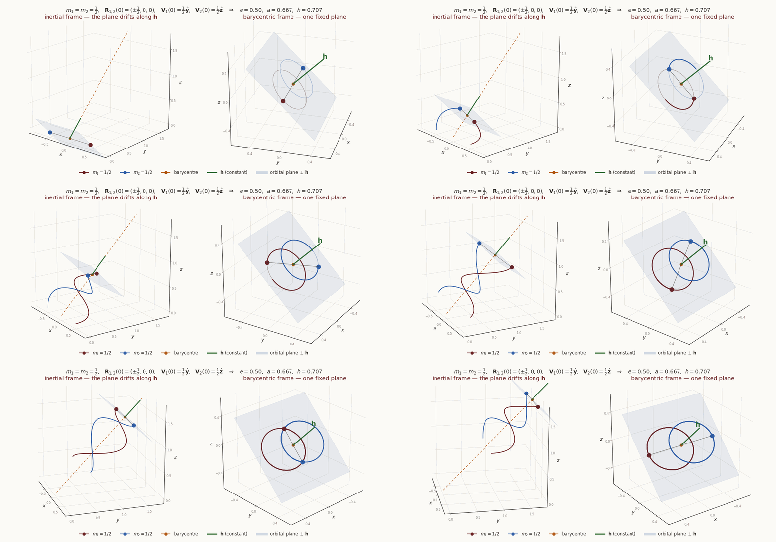
The bodies sit on the \(x\)-axis, equidistant from the origin; one is launched along \(y\), the other along \(z\). The separation lies along one axis and the two velocities along the other two — all three directions mutually perpendicular.
Clearly, the total linear momentum
\[
\mathbf{P} = m_1\mathbf{V}_1 + m_2\mathbf{V}_2 = \tfrac{1}{4}\left(\hat{\mathbf{y}} + \hat{\mathbf{z}}\right) \neq \mathbf{0}
\]
does not vanish, so the barycentre drifts. This is not the tidy equal-and-opposite setup of the previous animation.
The orbit, before any integration
The relative state at \(t = 0\) is
\[
\mathbf{r}(0) = \mathbf{R}_2 - \mathbf{R}_1 = -\hat{\mathbf{x}}, \qquad
\dot{\mathbf{r}}(0) = \mathbf{V}_2 - \mathbf{V}_1 = \tfrac{1}{2}\left(\hat{\mathbf{z}} - \hat{\mathbf{y}}\right),
\]
so the integrals are fixed once and for all by these two vectors:
\[
\mathbf{h} = \mathbf{r} \times \dot{\mathbf{r}} = \tfrac{1}{2}\left(\hat{\mathbf{y}} + \hat{\mathbf{z}}\right),
\qquad h = \tfrac{1}{\sqrt{2}}, \qquad
\varepsilon = \frac{v^{2}}{2} - \frac{\mu}{r} = \frac{1}{4} - 1 = -\frac{3}{4},
\]
and — borrowing three results we shall derive in the next few slides (vis-viva, the period, and the second Casimir relation) — the whole geometry follows without solving anything:
\[
a = -\frac{\mu}{2\varepsilon} = \frac{2}{3}, \qquad
e = \sqrt{1 + \frac{2\varepsilon h^{2}}{\mu^{2}}} = \frac{1}{2}, \qquad
T = 2\pi\sqrt{\frac{a^{3}}{\mu}} = 3.4201 .
\]
Since \(\mathbf{r}\cdot\dot{\mathbf{r}} = 0\) at \(t = 0\), the run starts at an apsis; and \(r(0) = 1 = a(1+e)\) identifies it as apoapsis.
Helices, not closed curves
One more feature of this choice of initial data, which the animation is about to make obvious. The barycentre travels at
\[
\mathbf{V}_{cm} = \frac{\mathbf{P}}{M} = \tfrac{1}{4}\left(\hat{\mathbf{y}} + \hat{\mathbf{z}}\right)
\qquad\text{while}\qquad
\mathbf{h} = \tfrac{1}{2}\left(\hat{\mathbf{y}} + \hat{\mathbf{z}}\right),
\]
so \(\mathbf{V}_{cm} \parallel \mathbf{h}\): the drift is along the normal of the orbital plane. The plane therefore slides through space like a sheet pushed face-first, and neither body ever returns to a point it has already visited — each traces a helix, even though the relative orbit is a closed ellipse of period \(T = 3.4201\).
Two bodies in 3D
![]()
Figure 2: Left: the inertial frame — the barycentre (amber) runs off along a straight line, dragging the orbital plane with it, and each body traces a helix. Right: the barycentric frame — the drift subtracted, the two bodies run on similar (here congruent, as \(m_1 = m_2\)) ellipses in one plane that never moves. Shaded patch: the plane \(\perp \mathbf{h}\). Integrated with adaptive RKF7(8), \(rtol = 10^{-12}\). Download the script.
Equation of the Orbit
We now want the explicit geometric shape of the orbit — \(r\) as a function of position angle. The cleanest route uses what we have already derived. We have \(\mathbf{h}\) (which fixes the orbital plane) and \(\mathbf{e}\) (which fixes the line of apsides). All we have to do is exploit a single dot-product identity to read off \(r(f)\).
Take the dot product of \(\mathbf{r}\) with the eccentricity-vector integral \(\dot{\mathbf{r}} \times \mathbf{h} = \mu(\hat{\mathbf{r}} + \mathbf{e})\):
\[
\mathbf{r} \cdot (\dot{\mathbf{r}} \times \mathbf{h}) = (\mathbf{r} \times \dot{\mathbf{r}}) \cdot \mathbf{h} = \mathbf{h} \cdot \mathbf{h} = h^2.
\]
On the right side, let \(f\) be the angle between \(\mathbf{e}\) and \(\mathbf{r}\) (the true anomaly):
\[
\mathbf{r} \cdot \mu(\hat{\mathbf{r}} + \mathbf{e}) = \mu(r + re\cos f).
\]
Equating and solving for \(r\) (Battin Eq. 3.20):
\[
\boxed{r = \frac{p}{1 + e\cos f}}, \qquad p = \frac{h^2}{\mu}.
\]
This is the polar equation of a conic section with focus at the origin. The single number \(e\) — the magnitude of the eccentricity vector — determines the qualitative shape of the orbit:
| \(0\) |
circle |
bound |
| \(0 < e < 1\) |
ellipse |
bound |
| \(e = 1\) |
parabola |
escape, zero energy |
| \(e > 1\) |
hyperbola |
escape, positive energy |
For \(e>0\) and \(h^2/\mu = \text{const}\), \(f=0\) yields minimum \(r\). We call this as periapsis. Similarly, \(f=\pi\) has maximum \(r\). This is termed as apoapsis.
This settles the question of the direction of \(\mathbf{e}\) as well.
- Since \(f\) is the angle between \(\mathbf{r}\) and \(\mathbf{e}\), \(f=0\) yields the direction of \(\mathbf{e}\).
\[
\boxed{\text{$\mathbf{e}$ always points in the direction of periapsis.}}
\]
The ellipse
![]()
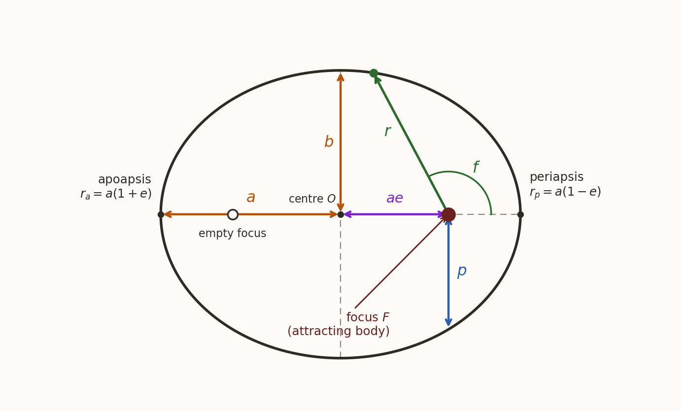
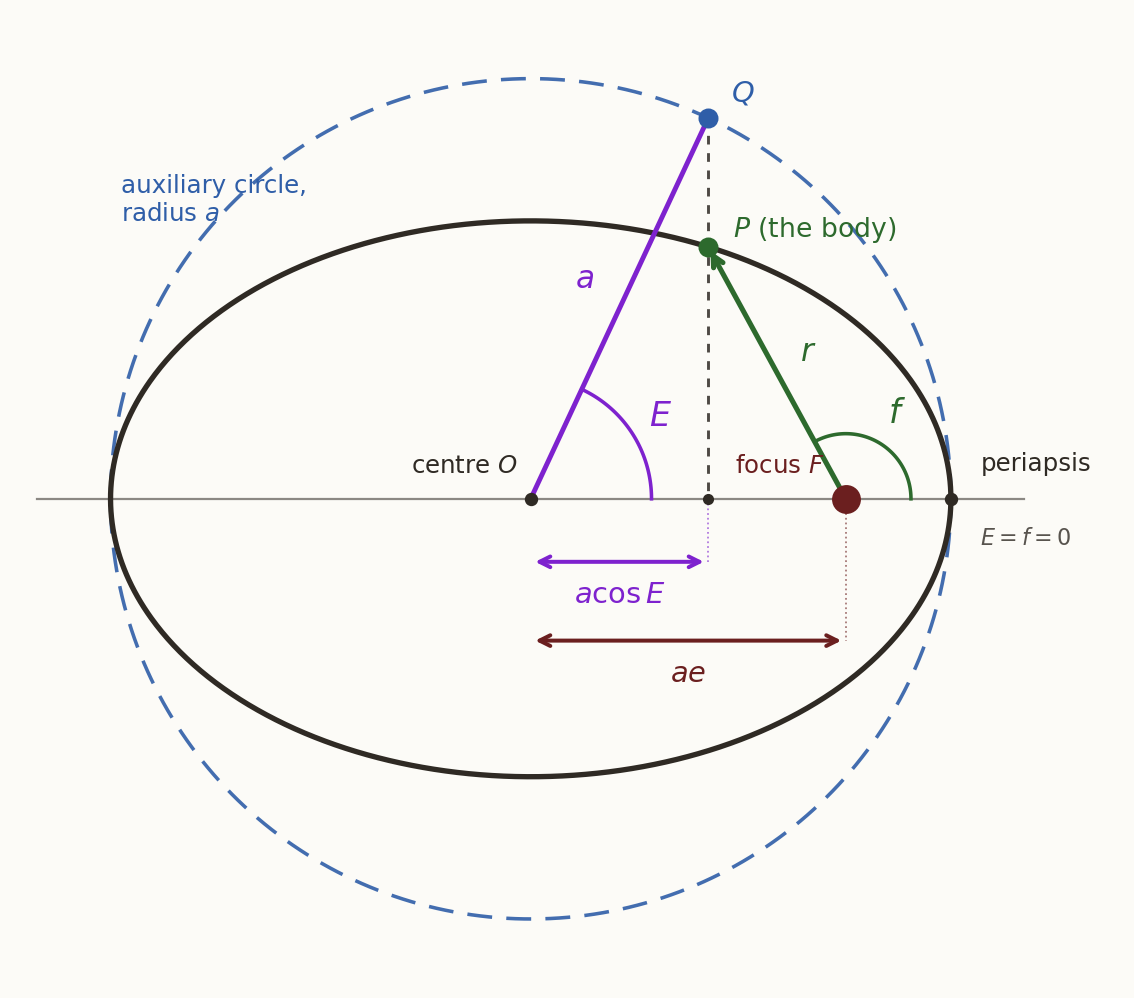
Figure 3: Geometry of the elliptic orbit (\(e = 0.6\)). The attracting body sits at the occupied focus \(F\); the other focus is empty. The centre-to-focus distance is \(ae\), so the eccentricity is the fractional offset of the focus from the centre. The semi-latus rectum \(p\) is the radius at \(f = \pi/2\), i.e. \(p = a(1-e^{2}) = b^{2}/a\), and the true anomaly \(f\) is measured at the focus from the periapsis direction.
Various Conic sections
All four numbers below describe the same orbit — move any one of them and watch the other three, and the curve, follow. Units are non-dimensional, with \(\mu = G(m_1+m_2) = 1\); the attracting body sits at the amber focus and periapsis is to the right.
Things to try
Hold \(h\) and sweep \(e\) from \(0\) to \(2.5\). Every curve in the family keeps the same semi-latus rectum \(p = h^{2}/\mu\) — the conic simply unrolls from circle to ellipse to parabola to hyperbola, and \(\varepsilon\) changes sign exactly at \(e = 1\).
Hold \(a\) (or, identically, \(\varepsilon\)) and sweep \(e\). Now the size is frozen: every ellipse has the same major axis, the same energy and the same period \(T\), but the focus slides from the centre out towards the periapsis. Energy is blind to shape.
Notice that the \(a\) and \(\varepsilon\) buttons do the same thing. They must: \(\varepsilon = -\mu/2a\) is a one-to-one map, so \((a, e)\) and \((\varepsilon, e)\) are the same parametrisation, and only \((h, e)\) is genuinely different.
Try to cross \(e = 1\) while holding \(a\). You cannot — the slider stops. An ellipse cannot become a hyperbola without \(a\) passing through infinity, which is the Casimir relation \(\mu^{2}\left(e^{2}-1\right) = 2\varepsilon h^{2}\) forbidding \(\operatorname{sign}\varepsilon \neq \operatorname{sign}(e-1)\). Hold \(h\) instead and the passage is smooth.
Two spacecraft are on orbits with the same \(a\) but \(e = 0.1\) and \(e = 0.9\). Which one is moving faster at periapsis, and which has the larger \(h\)?
Answer
\[
v_p = \sqrt{\frac{\mu}{a}}\,\sqrt{\frac{1+e}{1-e}}, \qquad
h = \sqrt{\mu a\left(1 - e^{2}\right)} .
\]
Faster at periapsis: \(e = 0.9\), and not narrowly — \(\sqrt{1.9/0.1} = 4.36\) against \(\sqrt{1.1/0.9} = 1.11\), a factor of \(3.9\).
Larger \(h\): the other one. \(\sqrt{1-e^{2}}\) is \(0.995\) for \(e = 0.1\) and only \(0.436\) for \(e = 0.9\).
So the eccentric orbit is much faster at periapsis yet carries less than half the angular momentum — because it is deep in (\(r_p = 0.1a\)) exactly when it is moving fast, and \(h = r_p v_p\). Equal \(a\) pins energy and period; it says nothing about \(h\).
Energy Integral (Vis-Viva)
We shall see, dotting the EOM with \(\dot{\mathbf{r}}\) produces a scalar conservation law — the energy integral, also known as the vis-viva (literally, “living force”) equation.
This is arguably the single most useful formula in mission design.
Dot-multiply the equation of motion by \(\dot{\mathbf{r}}\):
\[
\dot{\mathbf{r}} \cdot \ddot{\mathbf{r}} = -\frac{\mu}{r^3}\,\mathbf{r}\cdot\dot{\mathbf{r}},
\]
\[
\frac{d}{dt}\!\left(\frac{v^2}{2}\right) = -\frac{\mu\dot{r}}{r^2} = \frac{d}{dt}\!\left(\frac{\mu}{r}\right).
\]
Integrating
\[
\frac{v^2}{2} - \frac{\mu}{r} = \varepsilon
\]
where \(\varepsilon\) is the constant of integration.
This is the first form of the vis-viva equation.
Orbit classification based on \(\varepsilon\)
Rearranging the vis-viva equation:
\[
\boxed{v^2=2\left(\varepsilon+\frac{\mu}{r}\right)}.
\]
Since,
\[
v^2\geq 0,
\]
This condition allows us to determine directly whether the radial distance \(r\) can become arbitrarily large.
Negative specific energy: \(\varepsilon<0\)
If the specific mechanical energy is negative, write
\[
\varepsilon=-|\varepsilon|.
\]
The vis-viva equation becomes
\[
v^2=2\left(\frac{\mu}{r}-|\varepsilon|\right).
\]
Since \(v^2\geq 0\),
\[
2\left(\frac{\mu}{r}-|\varepsilon|\right)\geq 0.
\]
Therefore,
\[
\frac{\mu}{r}\geq |\varepsilon|.
\]
Because \(r>0\) and \(|\varepsilon|>0\), this gives
\[
r\leq\frac{\mu}{|\varepsilon|}.
\]
Thus, there is a finite upper limit on the distance from the attracting body. Consequently,
\[
\boxed{\varepsilon<0\quad\Longrightarrow\quad\text{bounded motion}.}
\]
Show that \(r \le 2a\) for any orbit with \(\varepsilon \le 0\).
Answer
From \(\varepsilon = \dfrac{v^{2}}{2} - \dfrac{\mu}{r}\) and \(v^{2} \ge 0\),
\[
\frac{\mu}{r} = \frac{v^{2}}{2} - \varepsilon \;\ge\; -\varepsilon = \frac{\mu}{2a}
\qquad\Longrightarrow\qquad r \le 2a .
\]
Equality demands \(v = 0\). A genuine orbit never stops, so for \(h \neq 0\) the bound is strict and the sharp value is \(r_a = a(1+e) < 2a\); the case that does attain it is the rectilinear orbit \(h = 0\), which comes to rest exactly at \(r = 2a\) before falling back.
(For \(\varepsilon = 0\), \(a \to \infty\) and the bound says nothing — correctly, since a parabola is unbounded.)
Positive specific energy: \(\varepsilon>0\)
For positive energy, vis-viva gives
\[
v^2=2\left(\varepsilon+\frac{\mu}{r}\right).
\]
\(\varepsilon > 0\) implies \(a \le 0\).
For every finite \(r>0\), both terms inside the parentheses are positive:
\[
\varepsilon>0,
\qquad
\frac{\mu}{r}>0.
\]
Therefore,
\[
v^2>0
\]
at every finite radius. In particular, there is no finite outer radius at which
\[
v=0.
\]
Thus, the energy equation imposes no upper bound on \(r\).
As \(r\to\infty\),
\[
\frac{\mu}{r}\to0,
\]
and hence
\[
v^2\to2\varepsilon.
\]
Taking the positive square root for speed,
\[
\boxed{v\to\sqrt{2\varepsilon}>0}.
\]
Therefore, the body can reach infinity while retaining a nonzero speed. This asymptotic speed is called the hyperbolic excess speed:
\[
\boxed{v_\infty=\sqrt{2\varepsilon}}.
\]
Consequently,
\[
\boxed{\varepsilon>0\quad\Longrightarrow\quad\text{unbounded motion}.}
\]
Zero specific energy: \(\varepsilon=0\)
The zero-energy case separates bounded and positive-energy unbounded motion. Setting \(\varepsilon=0\) in vis-viva gives
\[
v^2=\frac{2\mu}{r}.
\]
For every finite \(r>0\), we have \(v^2>0\). Therefore, there is no finite outer turning point.
As \(r\to\infty\), \(v^2\to0\) and hence \(v\to0\). Thus the body can reach infinity, but its speed approaches zero:
\[
\boxed{\varepsilon=0\quad\Longrightarrow\quad\text{marginally unbounded motion}.}
\]
This is the parabolic escape condition.
Evaluating \(\varepsilon\)
Since \(\varepsilon\) is constant, we may evaluate it anywhere on the orbit. Periapsis is the cheapest point: there \(\dot r = 0\), the velocity is purely transverse, and hence \(h = r_p v_p\), i.e. \(v_p = h/r_p\):
\[
\varepsilon = \frac{v_p^{2}}{2} - \frac{\mu}{r_p} = \frac{h^{2}}{2 r_p^{2}} - \frac{\mu}{r_p}.
\]
Substituting \(h^{2} = \mu a\left(1 - e^{2}\right)\) and \(r_p = a(1-e)\) from the previous slide:
\[
\begin{aligned}
\varepsilon
&= \frac{\mu a\left(1 - e^{2}\right)}{2 a^{2}(1-e)^{2}} - \frac{\mu}{a(1-e)}
= \frac{\mu (1+e)}{2 a (1-e)} - \frac{\mu}{a(1-e)} \\[4pt]
&= \frac{\mu}{a(1-e)}\left[\frac{1+e}{2} - 1\right]
= \frac{\mu}{a(1-e)} \cdot \frac{e-1}{2}
= -\frac{\mu}{2a}.
\end{aligned}
\]
The constant is therefore fixed by the size of the orbit alone:
\[
\boxed{\;\frac{v^{2}}{2} - \frac{\mu}{r} = -\frac{\mu}{2a}\;}
\qquad\Longleftrightarrow\qquad
\boxed{\;v^{2} = \mu\left(\frac{2}{r} - \frac{1}{a}\right)\;}
\]
This is the vis-viva equation in its working form.
Two orbits with the same \(a\) but wildly different shapes carry exactly the same energy — and, as we have just seen, the same period \(T = 2\pi\sqrt{a^{3}/\mu}\). Energy is blind to shape.
Putting \(a = r\) (a circle) we get the circular speed \(v_c = \sqrt{\mu/r}\)
\(\varepsilon = 0\) (\(a \to \infty\)) gives us the escape speed \(v_{esc} = \sqrt{2\mu/r} = \sqrt{2}\, v_c\).
Summary
| ellipse |
\(\varepsilon<0\) |
\(r\leq \mu/|\varepsilon|\) |
\(a > 0\) |
| parabola |
\(\varepsilon=0\) |
\(r\to\infty\) and \(v\to0\) |
\(a \to \infty\) |
| hyperbola |
\(\varepsilon>0\) |
\(r\to\infty\) and \(v\to\sqrt{2\varepsilon}\) |
\(a < 0\) |
Period (\(T\)) of an orbit
Step 1 — the areal velocity. With \(\mathbf{r} = r\hat{\mathbf{r}}\) and \(\dot{\mathbf{r}} = \dot r\,\hat{\mathbf{r}} + r\,\dot{\hat{\mathbf{r}}}\) (used earlier in the eccentricity-vector derivation),
\[
\mathbf{h} = \mathbf{r} \times \dot{\mathbf{r}}
= r\hat{\mathbf{r}} \times \left(\dot r\,\hat{\mathbf{r}} + r\,\dot{\hat{\mathbf{r}}}\right)
= r^{2}\,\hat{\mathbf{r}} \times \dot{\hat{\mathbf{r}}} .
\]
Because \(\mathbf{e}\) is a fixed vector, the apsidal line does not move, so the true anomaly \(f\) is the polar angle of \(\hat{\mathbf{r}}\): writing \(\dot{\hat{\mathbf{r}}} = \dot f\,\hat{\boldsymbol{\theta}}\) with \(\hat{\boldsymbol{\theta}} \perp \hat{\mathbf{r}}\) in the orbital plane,
\[
h = r^{2}\dot f .
\]
The radius vector sweeps a thin sector of area \(dA = \tfrac{1}{2} r^{2}\,df\), hence
\[
\frac{dA}{dt} = \frac{1}{2} r^{2}\dot f = \frac{h}{2} = \text{const},
\]
which is Kepler’s second law once more. Constant rate is the whole point: the area is swept uniformly, so one revolution can be timed by simple division.
Step 2 — the area enclosed. For an ellipse \(A = \pi a b\), so we need \(b\); and \(b\) follows from the orbit equation alone. Put \(\cos f = -e\) in \(r = a(1-e^{2})/(1 + e\cos f)\):
\[
r = \frac{a\left(1 - e^{2}\right)}{1 - e^{2}} = a,
\qquad
r\cos f = -ae .
\]
That point lies a distance \(ae\) to the left of the focus; but the centre is itself \(ae\) to the left of the focus (Figure 3), so the point sits directly above the centre — it is the end of the minor axis. By Pythagoras,
\[
b^{2} = a^{2} - (ae)^{2}
\qquad \Longrightarrow \qquad
b = a\sqrt{1 - e^{2}} = \sqrt{a p} .
\]
Step 3 — divide. One revolution sweeps the whole ellipse at the constant rate \(h/2\):
\[
T = \frac{A}{dA/dt} = \frac{\pi a b}{h/2}
= \frac{2\pi\, a \cdot a\sqrt{1 - e^{2}}}{\sqrt{\mu a \left(1 - e^{2}\right)}}
= \frac{2\pi a^{2}}{\sqrt{\mu a}},
\]
\[
\boxed{\;T = 2\pi\sqrt{\frac{a^{3}}{\mu}}\;}
\qquad\qquad
n \equiv \frac{2\pi}{T} = \sqrt{\frac{\mu}{a^{3}}}
\]
where \(n\) is the mean motion, the average angular rate — the quantity we shall need when we come to Kepler’s equation.
Note once again that \(e\) has cancelled: the period, like the energy, depends only on \(a\). Indeed \(T\) and \(\varepsilon = -\mu/2a\) are two readings of the same number. And \(T\) exists only for \(a > 0\): a parabola or hyperbola never closes.
Kepler’s third law Modification
Squaring, \(T^{2} = \dfrac{4\pi^{2}}{G(m_1 + m_2)}\,a^{3}\). Kepler asserted \(T^{2} \propto a^{3}\) with the same constant for every planet; Newton’s version shows the constant carries \(m_1 + m_2\). For the Sun and even its heaviest planet \(m_2/m_1 \approx 10^{-3}\), so the discrepancy is a few parts in \(10^{4}\) — comfortably below Kepler’s observational precision, which is why he never saw it.
Casimir relations
We have now squeezed the two-body equation of motion three different ways — cross product, BAC–CAB, dot product — and harvested three integrals:
\[
\mathbf{h} = \mathbf{r} \times \dot{\mathbf{r}}, \qquad
\mathbf{e} = \frac{\dot{\mathbf{r}} \times \mathbf{h}}{\mu} - \frac{\mathbf{r}}{r}, \qquad
\varepsilon = \frac{v^2}{2} - \frac{\mu}{r}
\]
That is \(3 + 3 + 1 = 7\) scalar constants for a system whose state has only \(6\) degrees of freedom. They cannot all be independent. Exactly two relations tie them together, and these are called the Casimir relations:
\[
\boxed{\;\mathbf{h} \cdot \mathbf{e} = 0\;}
\qquad\qquad
\boxed{\;\mu^{2}\left(e^{2} - 1\right) = 2\,\varepsilon\, h^{2}\;}
\]
Neither is a new integral. They are identities — constraints satisfied by the integrals we already have, at every instant, on every orbit.
First relationship is trivial. So we will prove the second.
Square the expression for \(\mathbf{e}\),
\[
\mu^{2} e^{2}
= \underbrace{\left| \dot{\mathbf{r}} \times \mathbf{h} \right|^{2}}_{\text{(i)}}
- 2\mu\, \underbrace{\hat{\mathbf{r}} \cdot \left( \dot{\mathbf{r}} \times \mathbf{h} \right)}_{\text{(ii)}}
+ \mu^{2}\, \underbrace{\hat{\mathbf{r}} \cdot \hat{\mathbf{r}}}_{= \,1}
\]
Term (i): \(\mathbf{h} = \mathbf{r} \times \dot{\mathbf{r}}\) is perpendicular to \(\dot{\mathbf{r}}\), so the cross product has magnitude \(v h\) with no \(\sin\) factor to worry about:
\[
\left| \dot{\mathbf{r}} \times \mathbf{h} \right|^{2} = v^{2} h^{2}
\]
Term (ii): cycle the triple product so that \(\mathbf{h}\) meets \(\mathbf{r} \times \dot{\mathbf{r}}\):
\[
\hat{\mathbf{r}} \cdot \left( \dot{\mathbf{r}} \times \mathbf{h} \right)
= \frac{1}{r}\, \mathbf{r} \cdot \left( \dot{\mathbf{r}} \times \mathbf{h} \right)
= \frac{1}{r}\, \mathbf{h} \cdot \left( \mathbf{r} \times \dot{\mathbf{r}} \right)
= \frac{h^{2}}{r}
\]
Substituting both terms,
\[
\mu^{2} e^{2}
= v^{2} h^{2} - \frac{2 \mu h^{2}}{r} + \mu^{2}
= h^{2} \left( v^{2} - \frac{2\mu}{r} \right) + \mu^{2}
\]
The bracket is precisely twice the specific energy, \(v^{2} - 2\mu/r = 2\varepsilon\). Hence
\[
\mu^{2} e^{2} = 2 \varepsilon h^{2} + \mu^{2}
\qquad \Longrightarrow \qquad
\mu^{2}\left( e^{2} - 1 \right) = 2 \varepsilon h^{2}
\]
or, solved for the eccentricity,
\[
e = \sqrt{1 + \frac{2 \varepsilon h^{2}}{\mu^{2}}}
\]
Since \(h^{2} \ge 0\) and \(\mu > 0\), the sign of \(\varepsilon\) alone decides the shape of the conic:
| \(\varepsilon < 0\) |
\(e < 1\) |
ellipse (bound) |
| \(\varepsilon = 0\) |
\(e = 1\) |
parabola (escape) |
| \(\varepsilon > 0\) |
\(e > 1\) |
hyperbola (unbound) |
This is why the vis-viva constant is the natural “mission design” variable: it tells you at a glance whether you are captured or escaping.
Substituting the vis-viva result \(\varepsilon = -\mu / (2a)\) into relation 2 gives
\[
\mu^{2}\left(e^{2} - 1\right) = -\frac{\mu h^{2}}{a}
\qquad \Longrightarrow \qquad
h^{2} = \mu\, a \left( 1 - e^{2} \right) = \mu\, p
\]
Here we have again arrived at the conic equation we already know.
Counting the integrals
The two Casimir relations settle the bookkeeping we started in the N-body section:
- We possess \(7\) scalar constants: \(\mathbf{h}\,(3)\), \(\mathbf{e}\,(3)\), \(\varepsilon\,(1)\).
- Relation 1 removes one; relation 2 removes another.
- That leaves \(5\) independent constants of the motion.
Five constants fix the orbit as a curve in space.
Its shape (\(a, e\)) or (\(\varepsilon, e\)) or (\(h, e\)).
What they cannot tell us is where on that curve the body is. One more constant, either in the form of \(f\) or time of perapsis passage (\(t_p\)) fixes the position.
\[
5 \;(\text{geometry}) \;+\; 1 \;(\text{timing, } t_p) \;=\; 6 \;=\; \text{order of the reduced system}
\]
Velocity
Goal for this deck: given that \(r(f)\) is known, obtain \(\mathbf{v}\) as an explicit function of the true anomaly \(f\) — magnitude and direction — without ever solving for \(t\).
The two ingredients
We will use exactly two facts, both already proved:
- The orbit equation. \(r = p/(1 + e\cos f)\), with \(f\) measured from periapsis at the focus.
- Angular momentum. \(h = r^{2}\dot f = \text{const}\), which is what converts any \(d/df\) into a \(d/dt\):
\[
\frac{d}{dt} = \dot f\,\frac{d}{df} = \frac{h}{r^{2}}\,\frac{d}{df} .
\]
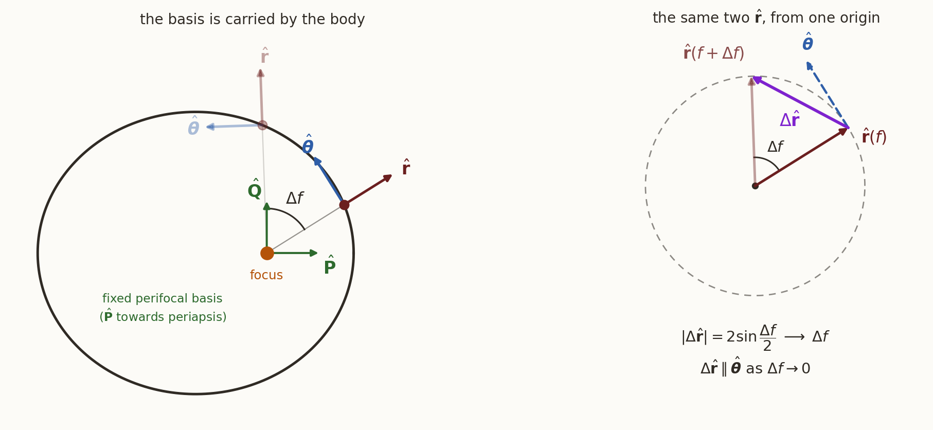
Working in the orbital plane with the rotating unit vectors \(\hat{\mathbf{r}}\) (radially outward) and \(\hat{\boldsymbol{\theta}}\) (transverse, in the direction of increasing \(f\)). They rotate with the body:
\[
\dot{\hat{\mathbf{r}}} = \dot f\,\hat{\boldsymbol{\theta}}, \qquad
\dot{\hat{\boldsymbol{\theta}}} = -\dot f\,\hat{\mathbf{r}} .
\]
Both statements are proved at the end of the deck — see the appendix, The rotating basis \((\hat{\mathbf{r}}, \hat{\boldsymbol{\theta}})\).
Differentiating \(\mathbf{r} = r\,\hat{\mathbf{r}}\),
\[
\mathbf{v} = \dot{\mathbf{r}} = \dot r\,\hat{\mathbf{r}} + r\dot f\,\hat{\boldsymbol{\theta}}
\;\equiv\; v_r\,\hat{\mathbf{r}} + v_\perp\,\hat{\boldsymbol{\theta}} .
\]
So there are only two numbers to find: the radial speed \(v_r = \dot r\) and the transverse speed \(v_\perp = r\dot f\).
\(v_r\) changes the size of \(\mathbf{r}\); \(v_\perp\) changes its direction. Only \(v_\perp\) carries angular momentum — indeed \(h = r v_\perp\).
The transverse component
Angular momentum gives it with no work at all:
\[
v_\perp = r\dot f = \frac{h}{r}
= \frac{h}{p}\left(1 + e\cos f\right) .
\]
Using \(p = h^{2}/\mu\), the prefactor is \(h/p = \mu/h\):
\[
\boxed{\;v_\perp = \frac{\mu}{h}\left(1 + e\cos f\right)\;}
\]
- \(v_\perp > 0\) everywhere the conic exists, since \(1 + e\cos f = p/r > 0\) — the body never reverses its swing.
- \(v_\perp\) is largest at periapsis and smallest at apoapsis, exactly as \(h = rv_\perp = \text{const}\) demands.
The radial component
Differentiate the orbit equation. It is cleanest in reciprocal form:
\[
\frac{1}{r} = \frac{1 + e\cos f}{p}
\qquad\Longrightarrow\qquad
-\frac{\dot r}{r^{2}} = -\frac{e\sin f}{p}\,\dot f .
\]
Hence
\[
\dot r = \frac{r^{2}\dot f}{p}\,e\sin f = \frac{h}{p}\,e\sin f ,
\]
where \(r^{2}\dot f = h\) was used in the very last step. With \(h/p = \mu/h\) again,
\[
\boxed{\;v_r = \frac{\mu}{h}\,e\sin f\;}
\]
Both components carry the same prefactor \(\mu/h = h/p = \sqrt{\mu/p}\). This is the natural speed unit of the orbit — the circular speed at radius \(p\). Every velocity formula below is that number times a pure function of \(e\) and \(f\).
The velocity vector
Putting the two together:
\[
\boxed{\;
\mathbf{v}(f) = \frac{\mu}{h}\left[\,e\sin f\;\hat{\mathbf{r}}
\;+\;\left(1 + e\cos f\right)\hat{\boldsymbol{\theta}}\,\right] \;}
\]
Clearly,
- \(v_r = 0\) at \(f = 0\) and \(f = \pi\) — the apsides are precisely the points where the radius stops growing or shrinking. The velocity there is purely transverse, i.e. perpendicular to \(\mathbf{r}\).
- \(v_r > 0\) on the outbound half \(0 < f < \pi\) and \(v_r < 0\) on the inbound half.
- \(e = 0\) kills \(v_r\) everywhere: circular motion, speed \(\sqrt{\mu/p}\), forever perpendicular to the radius.
The speed
\[
v^{2} = v_r^{2} + v_\perp^{2}
= \frac{\mu^{2}}{h^{2}}\left[e^{2}\sin^{2}f + \left(1 + e\cos f\right)^{2}\right] .
\]
Expand the bracket:
\[
e^{2}\sin^{2}f + 1 + 2e\cos f + e^{2}\cos^{2}f = 1 + 2e\cos f + e^{2} .
\]
So, using \(\mu^2/h^2 = \mu/p\),
\[
\boxed{\;v(f) = \sqrt{\frac{\mu}{p}}\;\sqrt{1 + 2e\cos f + e^{2}}\;}
\]
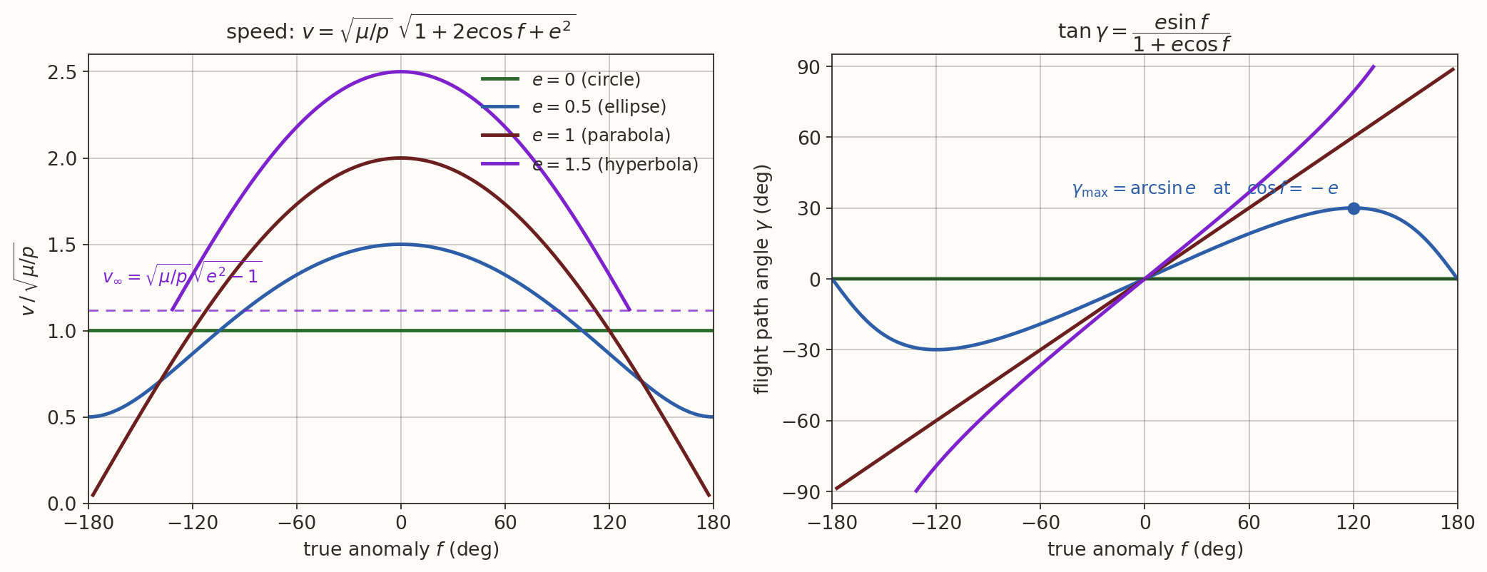
The speed depends on \(f\) only through \(\cos f\), so it is symmetric about the apse line — the body passes any given radius on the way out and on the way in with the same speed, and with flight path angles equal and opposite.
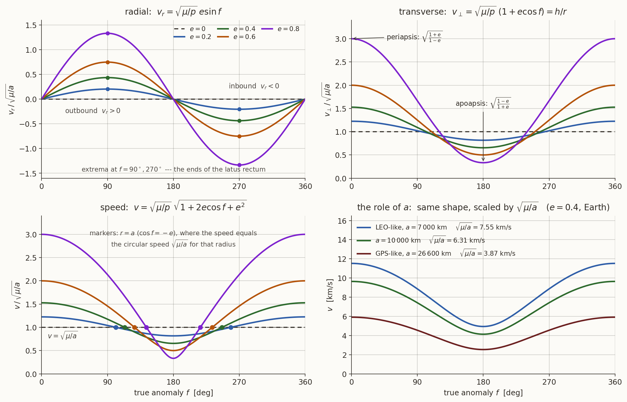
The three speeds, plotted
Divide every component by \(\sqrt{\mu/a}\) and the semi-major axis disappears:
\[
\frac{v_r}{\sqrt{\mu/a}} = \frac{e\sin f}{\sqrt{1-e^{2}}}, \qquad
\frac{v_\perp}{\sqrt{\mu/a}} = \frac{1 + e\cos f}{\sqrt{1-e^{2}}}, \qquad
\frac{v}{\sqrt{\mu/a}} = \frac{\sqrt{1 + 2e\cos f + e^{2}}}{\sqrt{1-e^{2}}} .
\]
So \(e\) fixes the shape of all three curves and \(a\) only sets the scale.
What the plot says
- Two knobs, and they do different jobs. \(e\) chooses the curve, \(a\) chooses the units. Two orbits of the same \(e\) have identical velocity histories up to the factor \(\sqrt{\mu/a}\) — which is why \(e\), not \(a\), is what makes an orbit “energetic” to fly.
- \(v_r\) is odd about the apse line. It vanishes at both apsides and is extremal at \(f = 90^{\circ}, 270^{\circ}\) — the ends of the latus rectum — where \(|v_r| = (\mu/h)\,e\). Outbound is the top half, inbound the bottom.
- \(v_\perp\) never changes sign. It is \(h/r\), so it is largest at periapsis and smallest at apoapsis, in the ratio
\[
\frac{v_{\perp,p}}{v_{\perp,a}} = \frac{1+e}{1-e} = \frac{r_a}{r_p},
\]
which is just \(h = r v_\perp = \text{const}\) read twice. - The apsidal speeds multiply to the circular value. At the apsides \(v = v_\perp\), and
\[
v_p = \sqrt{\frac{\mu}{a}}\sqrt{\frac{1+e}{1-e}}, \qquad
v_a = \sqrt{\frac{\mu}{a}}\sqrt{\frac{1-e}{1+e}}, \qquad
v_p\,v_a = \frac{\mu}{a} .
\]
- The speed equals \(\sqrt{\mu/a}\) exactly where \(r = a\), i.e. at \(\cos f = -e\) (the ends of the minor axis) — marked on the third panel. Vis-viva says so at a glance: \(v^{2} = \mu(2/r - 1/a) = \mu/a\) when \(r = a\). Inside that radius the body is faster than a circular orbit of the same radius would be, outside it slower. It is also, as the next slide shows, where the velocity is tilted furthest from the horizon.
- Eccentric orbits are lopsided in time as well as speed. As \(e \to 1\) at fixed \(a\), \(v_p \sim \sqrt{2\mu/(a(1-e))} \to \infty\) while \(v_a \to 0\): the body hurries through periapsis and loiters at apoapsis. That is Kepler’s second law seen from the velocity side.
Flight Path Angle (\(\gamma\))
The flight path angle \(\gamma\) is the angle between the velocity and the local horizon — the direction perpendicular to \(\mathbf{r}\), i.e. \(\hat{\boldsymbol{\theta}}\). It is positive when the body is climbing.
\[
\tan\gamma = \frac{v_r}{v_\perp}, \qquad
\cos\gamma = \frac{v_\perp}{v} = \frac{h}{r v}, \qquad
\sin\gamma = \frac{v_r}{v} .
\]
Substituting the two components derived above, the common factor \(\mu/h\) cancels:
\[
\boxed{\;\tan\gamma(f) = \frac{e\sin f}{1 + e\cos f}\;}
\]
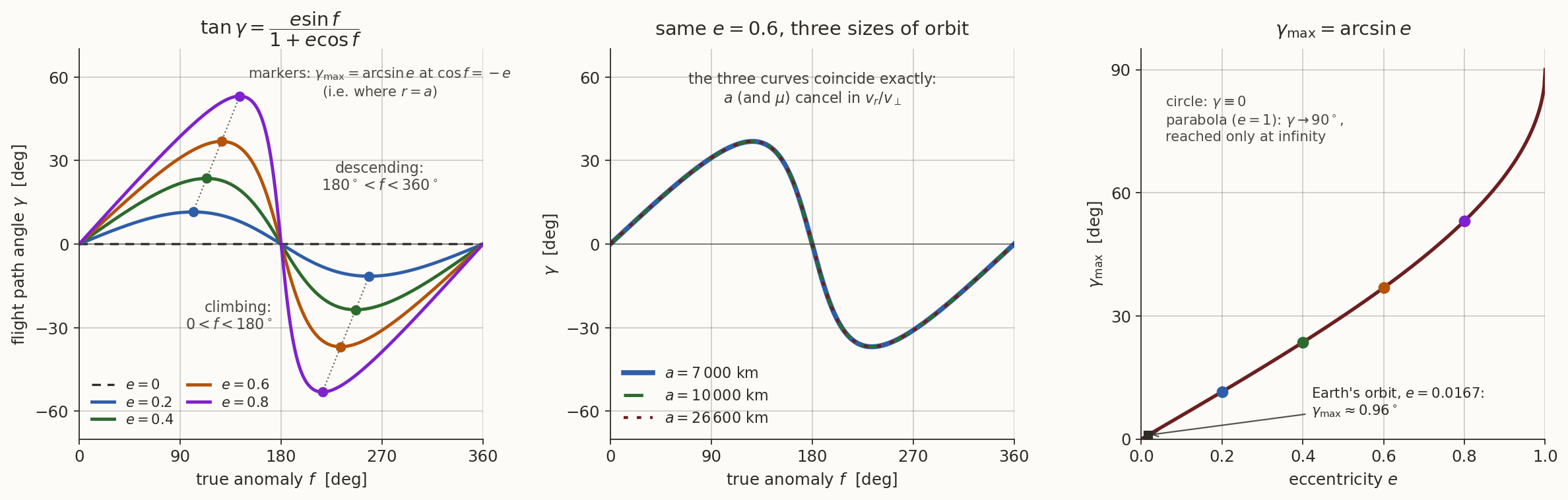
Only \(e\) and \(f\) survive. Neither \(a\) nor \(\mu\) nor \(h\) appears — \(\gamma\) is a ratio of two velocity components that carry the same prefactor. Scale the orbit up (\(a\)) or change the central body (\(\mu\)): the direction of flight at a given true anomaly does not move.
Where \(\gamma\) is zero, and where it is largest
At the apsides \(\sin f = 0\), so \(\gamma = 0\): the velocity is purely transverse and \(v = h/r\) there — the two points where speed and radius decouple.
For the maximum, differentiate the tangent:
\[
\frac{d}{df}\!\left(\frac{e\sin f}{1 + e\cos f}\right)
= \frac{e\cos f\,(1 + e\cos f) + e^{2}\sin^{2} f}{(1 + e\cos f)^{2}}
= \frac{e\,(\cos f + e)}{(1 + e\cos f)^{2}} ,
\]
which vanishes at \(\cos f = -e\). There \(\sin f = \sqrt{1-e^{2}}\) and \(1 + e\cos f = 1 - e^{2}\), so
\[
\tan\gamma_{\max} = \frac{e\sqrt{1-e^{2}}}{1-e^{2}} = \frac{e}{\sqrt{1-e^{2}}}
\qquad\Longrightarrow\qquad
\boxed{\;\gamma_{\max} = \arcsin e\;}
\]
- The location \(\cos f = -e\) is exactly \(r = p/(1-e^{2}) = a\): the ends of the minor axis. Same point as on the previous slide — where \(v = \sqrt{\mu/a}\), the velocity is also tilted furthest from the horizon.
- \(\gamma > 0\) on the outbound half, \(\gamma < 0\) on the inbound half, with equal and opposite values at the same radius. A circle has \(\gamma \equiv 0\).
- \(h = r v \cos\gamma\) is the practical form: with a radar range, a range rate and a speed you have the angular momentum, and the orbit follows.
\(\gamma\) across a family of ellipses
- \(a\) does nothing to \(\gamma\); \(e\) does everything. Raising the orbit changes every speed but not a single flight path angle.
- Near-circular orbits fly nearly horizontally. For small \(e\), \(\gamma \approx e\sin f\), so the Earth’s orbit (\(e = 0.0167\)) never tilts more than about \(0.96^{\circ}\) — which is why “circular” is such a good first approximation for planets and for most operational satellites.
- \(\gamma_{\max} = \arcsin e\) grows slowly at first (\(e = 0.2\) gives only \(11.5^{\circ}\)) and then sharply: \(e = 0.8\) gives \(53^{\circ}\), and the parabolic limit \(e \to 1\) approaches \(90^{\circ}\) — radial escape, all climb and no swing.
Picture
Velocity Hodograph
The component form hides something remarkable. Go back to the eccentricity-vector integral,
\[
\dot{\mathbf{r}}\times\mathbf{h} = \mu\left(\hat{\mathbf{r}} + \mathbf{e}\right),
\]
and cross it with \(\mathbf{h}\) from the left. Using \(\mathbf{h}\times(\mathbf{v}\times\mathbf{h}) = h^{2}\mathbf{v} - \mathbf{h}(\mathbf{h}\cdot\mathbf{v})\) and \(\mathbf{h}\cdot\mathbf{v} = 0\),
\[
\boxed{\;\mathbf{v} = \frac{\mu}{h}\,\hat{\mathbf{h}}\times\left(\hat{\mathbf{r}} + \mathbf{e}\right)\;}
\]
Now read it: \(\hat{\mathbf{h}}\times\) is just a \(90^{\circ}\) rotation inside the orbital plane. So \(\mathbf{v}\) is
\[
\underbrace{\frac{\mu}{h}\,\hat{\mathbf{h}}\times\hat{\mathbf{r}}}_{\text{unit vector, rotating with }f}
\;+\;
\underbrace{\frac{\mu}{h}\,\hat{\mathbf{h}}\times\mathbf{e}}_{\text{fixed vector}} .
\]
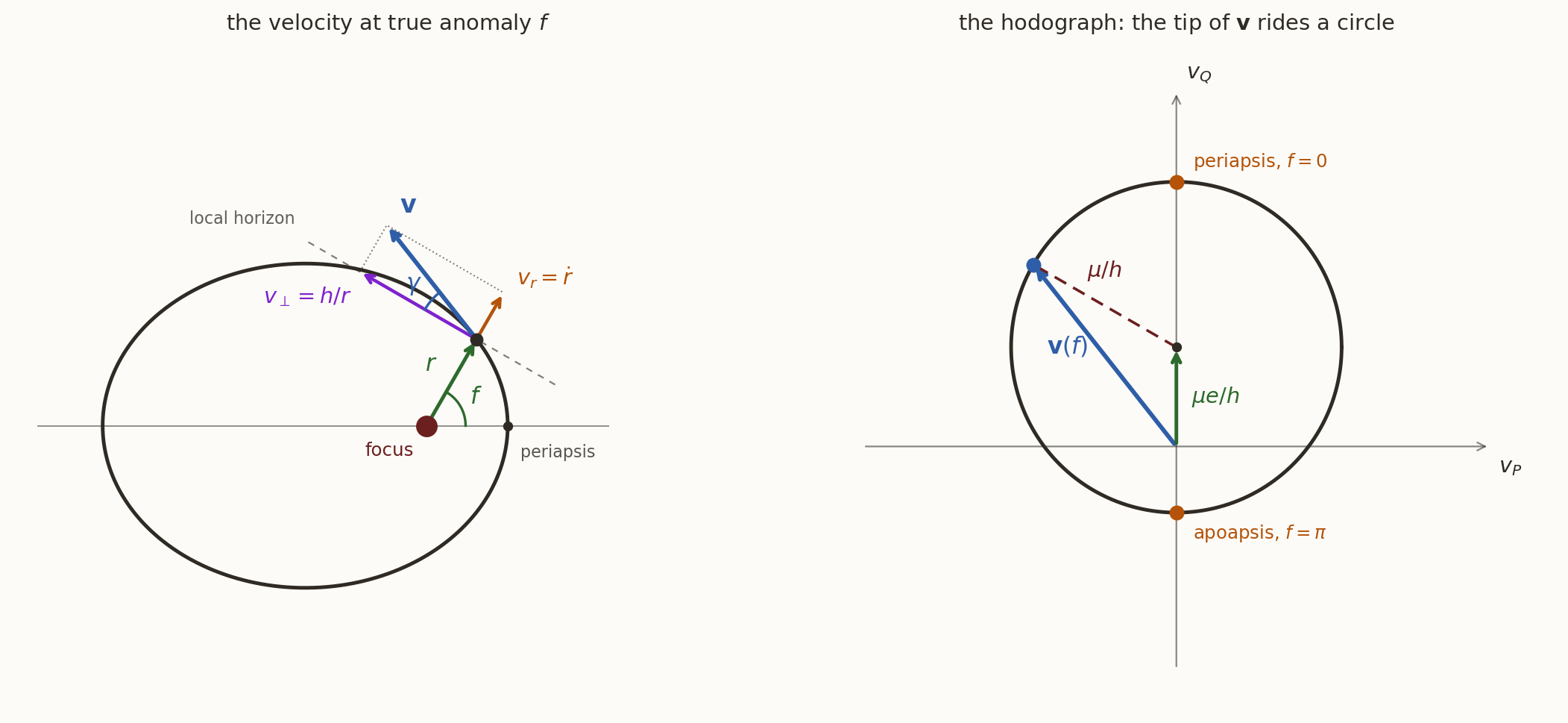
A vector of constant length \(\mu/h\) sweeping a full turn, added to a constant vector. The tip of \(\mathbf{v}\) therefore moves on a circle of radius \(\mu/h\) centred at distance \(\mu e/h\) from the origin of velocity space, perpendicular to \(\mathbf{e}\). This curve is the hodograph.
The hodograph in components
In the perifocal frame \((\hat{\mathbf{P}}\) towards periapsis, \(\hat{\mathbf{Q}}\) at \(90^{\circ}\) in the direction of motion\()\), substituting \(\hat{\mathbf{r}} = \cos f\,\hat{\mathbf{P}} + \sin f\,\hat{\mathbf{Q}}\):
\[
\boxed{\;
v_P = -\frac{\mu}{h}\sin f, \qquad
v_Q = \frac{\mu}{h}\left(e + \cos f\right) \;}
\]
\[
\Longrightarrow\quad
v_P^{2} + \left(v_Q - \frac{\mu e}{h}\right)^{2} = \left(\frac{\mu}{h}\right)^{2} .
\]
- Every Kepler orbit — ellipse, parabola or hyperbola — has a circular hodograph. Only the portion traversed differs: the ellipse goes round and round, the hyperbola covers only the arc \(|f| < \arccos(-1/e)\) and the two missing endpoints are the incoming and outgoing \(\mathbf{v}_\infty\).
- \(e < 1\) puts the velocity-space origin inside the circle (every direction of flight is achieved); \(e > 1\) puts it outside (the flight direction is confined to a wedge — the turning angle of a flyby).
Hamilton published the circularity of the hodograph in 1846 and used it to give a purely geometric proof of Kepler’s laws; Möbius and Maxwell used it as a teaching device. It is the cleanest statement of “the inverse-square law is special”.
Speed and flight path angle across the conics
Apsidal speeds
Put \(f = 0\) and \(f = \pi\) in the boxed speed formula:
\[
v_p = \sqrt{\frac{\mu}{p}}\left(1 + e\right)
= \sqrt{\frac{\mu}{a}\,\frac{1+e}{1-e}}, \qquad
v_a = \sqrt{\frac{\mu}{p}}\left(1 - e\right)
= \sqrt{\frac{\mu}{a}\,\frac{1-e}{1+e}} .
\]
Two consequences worth remembering:
\[
\frac{v_p}{v_a} = \frac{1+e}{1-e} = \frac{r_a}{r_p},
\qquad
v_p\,v_a = \frac{\mu}{p}\left(1-e^{2}\right) = \frac{\mu}{a} = n^{2}a^{2} .
\]
The first is just \(h = rv\) at the apsides (angular momentum). The second says the geometric mean of the apsidal speeds is the circular speed at radius \(a\).
An orbit is raised by a small burn \(\Delta v\) applied horizontally at periapsis. Using \(v_p = \sqrt{\mu/p}\,(1+e)\) and \(h = r_pv_p\), show that \(r_a\) changes far more than \(r_p\) does. Where does the extra energy go?
Answer
The impulse is tangential at periapsis, so the burn point stays on the new orbit and is still its periapsis — the velocity is still perpendicular to \(\mathbf{r}\), and the speed there has only gone up. Hence
\[\delta r_p = 0 ,\]
and the whole change is forced onto the far side. With \(\varepsilon = -\mu/2a\) and \(\delta\varepsilon = v_p\,\delta v\),
\[
\delta a = \frac{2a^{2}}{\mu}\,v_p\,\delta v ,
\qquad
r_a = 2a - r_p
\;\Longrightarrow\;
\delta r_a = 2\,\delta a = \frac{4a^{2}v_p}{\mu}\,\delta v .
\]
For a LEO-sized orbit that coefficient is about \(3400\ \mathrm{km}\) per \(\mathrm{km\,s^{-1}}\): apoapsis does all the moving.
The energy goes into potential energy on the far side — the apoapsis climbs. And the leverage \(4a^{2}v_p/\mu\) grows with \(v_p\), which is the Oberth effect seen from the geometry side.
Limiting cases
| circle |
\(0\) |
\(\sqrt{\mu/a}\), constant |
\(0\) |
circle centred at origin |
| ellipse |
\(0<e<1\) |
\(\sqrt{\mu/p}\sqrt{1+2e\cos f + e^{2}}\) |
\(\lvert\gamma\rvert\le\arcsin e\) |
origin inside |
| parabola |
\(1\) |
\(\sqrt{2\mu/r} = 2\sqrt{\mu/p}\,\left|\cos\tfrac f2\right|\) |
\(f/2\) |
origin on the circle |
| hyperbola |
\(>1\) |
as above, \(\to v_\infty\) |
\(\to\) asymptote value |
origin outside |
For the hyperbola, at \(\cos f = -1/e\),
\[
v_\infty^{2} = \frac{\mu}{p}\left(1 - 2 + e^{2}\right) = \frac{\mu}{p}\left(e^{2}-1\right)
= \frac{\mu}{|a|} = C_3 ,
\]
recovering the characteristic energy from the escape-velocity slide.
Worked example — a GTO
A geostationary transfer orbit: perigee altitude \(300\) km, apogee at the geostationary radius. With \(\mu_\oplus = 3.986\times10^{5}\ \mathrm{km^{3}/s^{2}}\),
\[
r_p = 6678\ \mathrm{km},\quad r_a = 42164\ \mathrm{km}
\;\Longrightarrow\;
a = \frac{r_p + r_a}{2} = 24421\ \mathrm{km},\quad
e = \frac{r_a - r_p}{r_a + r_p} = 0.7266 .
\]
\[
v_p = \sqrt{\frac{\mu}{a}\frac{1+e}{1-e}} = 10.15\ \mathrm{km/s},
\qquad
v_a = 1.608\ \mathrm{km/s},
\qquad \frac{v_p}{v_a} = 6.31 = \frac{r_a}{r_p}\ \checkmark
\]
The steepest climb occurs at \(\cos f = -e\), i.e. \(f = 136.6^{\circ}\), where \(\gamma = \arcsin 0.7266 = 46.6^{\circ}\), \(r = a = 24421\) km and \(v = \sqrt{\mu/a} = 4.04\) km/s.
At which true anomaly is the spacecraft moving at exactly the local circular speed \(\sqrt{\mu/r}\)? (Hint: set \(v^{2} = \mu/r\) in vis-viva — the answer is \(r = a\), the same point as \(\gamma_{\max}\). Coincidence?)
Answer
Vis-viva gives \(v^{2} = \mu\!\left(\frac{2}{r} - \frac{1}{a}\right) =
\frac{\mu}{r}\), i.e. \(\frac{1}{r} = \frac{1}{a}\), so \(r = a\). Then
\[
1 + e\cos f = \frac{p}{a} = 1 - e^{2}
\qquad\Longrightarrow\qquad
\boxed{\cos f = -e}
\]
— two points, symmetric about the apse line: the ends of the minor axis, each exactly \(a\) from both foci.
Not a coincidence. From \(\tan\gamma = \dfrac{e\sin f}{1 + e\cos f}\),
\[
\frac{d}{df}\tan\gamma = \frac{e\,\left(\cos f + e\right)}{\left(1 + e\cos f\right)^{2}} = 0
\qquad\Longleftrightarrow\qquad \cos f = -e ,
\]
the same condition. Both are the single fact \(r = a\): inside that radius the body outruns a circular orbit of the same radius, outside it lags, and the crossing is where the velocity leans furthest from the local horizon.
Escape Velocity
For a body at distance \(r\) from a primary of gravitational parameter \(\mu\), the escape speed \(v_{esc}(r)\) is the least speed at which the body, moving under the two-body gravitational field alone, has a trajectory that is unbounded — i.e. \(r(t)\to\infty\) rather than returning to a finite apoapsis.
- Clearly that is parabolic trajectory.
The criterion is energetic, not kinematic. From the vis-viva equation,
\[
\varepsilon = \frac{v^{2}}{2} - \frac{\mu}{r},
\]
and \(\varepsilon\) is constant along the orbit. Two one-line arguments settle it:
If \(\varepsilon < 0\): since \(v^2 \ge 0\), we need \(\mu/r \ge -\varepsilon\), hence \(r \le \mu/(-\varepsilon) = 2a\). The motion is trapped inside a sphere — bounded. (Indeed \(r_a = a(1+e) \le 2a\).) If \(\varepsilon \ge 0\): then \(v^{2} = 2\varepsilon + 2\mu/r > 0\) for all finite \(r\), so the body never comes to rest; past periapsis it recedes without a turning point. So escape \(\iff \varepsilon \ge 0\), and the threshold \(\varepsilon = 0\) gives
\[
\boxed{\;v_{esc}(r) = \sqrt{\frac{2\mu}{r}} = \sqrt{2}\,v_c(r)\;}
\]
the marginal case being the parabolic orbit (\(e = 1\), \(a \to \infty\)).
It is a speed, not a velocity. The name is a historical misnomer. \(\varepsilon\) depends on \(|\mathbf{v}|\) only, so the escape condition is indifferent to direction — straight up, sideways, or \(45^\circ\) all escape at the same \(11.2\) km/s, provided the trajectory does not intersect the planet’s surface or atmosphere. Direction changes where you go, not whether you leave.
It is local: \(v_{esc}\) is a function of \(r\). “The escape velocity of Earth is 11.2 km/s” is shorthand for at Earth’s surface. From LEO (\(r \approx 6{,}700\) km) it is \(10.9\) km/s; from GEO, \(4.35\) km/s.
It is escape from one primary. Leaving Earth is not leaving the Sun. Escape from the Solar System starting at Earth’s orbit needs \(v_{esc} = \sqrt{2\mu_\odot/1\,\text{AU}} = 42.1\) km/s heliocentric
Excess speed is what mission design actually buys. If \(v > v_{esc}\) the orbit is hyperbolic and the residual speed at infinity is
\[ v_\infty^{2} = 2\varepsilon = v^{2} - v_{esc}^{2}, \qquad C_3 \equiv v_\infty^2 = -\mu/a,
\]
the characteristic energy \(C_3\) quoted on every launch-vehicle performance chart. Note \(v_\infty^2\) is the difference of squares, not of speeds — a small \(\Delta v\) above escape is disproportionately cheap (the Oberth effect in disguise).
From \(r(f)\) to \(r(t)\)
We still just have the trajectory and not the exact location on the trajectory.
We currently know \(r(f)\). We need \(r(t)\). So clearly, we need \(f(t)\).
Since,
\[
h = r^{2}\dot f
\qquad\Longrightarrow\qquad
dt = \frac{r^{2}}{h}\,df,
\]
substituting the orbit equation \(r = p/(1 + e\cos f)\) and integrating from periapsis (\(f = 0\) at \(t = t_p\)),
\[
t - t_p = \frac{p^{2}}{h}\int_{0}^{f} \frac{df'}{\left(1 + e\cos f'\right)^{2}} .
\]
This is the Kepler problem, and the integral is the obstruction. It is elementary, but ugly in \(f\) — and, worse, the answer cannot be inverted to give \(f(t)\) in closed form. The classical remedy is not to fight the integral but to change the variable.
Circumscribe the ellipse with its auxiliary circle: the circle of radius \(a\) centred at the ellipse’s centre \(O\). Drop a perpendicular from the orbiting point \(P\) to the major axis and extend it to meet the circle at \(Q\). The eccentric anomaly \(E\) is the angle \(Q\) subtends at the centre, measured from periapsis — whereas the true anomaly \(f\) is measured at the focus.
Clearly, \(Q = (a\cos E,\; a\sin E)\). Now we try to calculate the coordinates of P. By definition, \(x_P = x_Q = a \cos E\). To calculate \(y_P\) we use the centre-based ellipse equation:
\[
\frac{x_P^{2}}{a^{2}} + \frac{y_P^{2}}{b^{2}} = 1
\;\xrightarrow{\;x_P \,=\, a\cos E\;}\;
\cos^{2}E + \frac{y_P^{2}}{b^{2}} = 1
\quad\Longrightarrow\quad
y_P^{2} = b^{2}\left(1 - \cos^{2}E\right) = b^{2}\sin^{2}E ,
\]
so \(y_P = b\sin E\). \(P = (a\cos E,\; b\sin E)\)
The focus lies at \((ae, 0)\) relative to \(O\), so measured from the focus
\[
x_P = a\left(\cos E - e\right), \qquad
y_P = b \sin E = a\sqrt{1 - e^{2}}\,\sin E .
\]
Now, \[
\begin{aligned}
r^{2} = x_P^{2} + y_P^{2}
&= a^{2}\left(\cos E - e\right)^{2} + a^{2}\left(1 - e^{2}\right)\sin^{2}E \\[2pt]
&= a^{2}\left[\cos^{2}E - 2e\cos E + e^{2} + \sin^{2}E - e^{2}\sin^{2}E\right] \\[2pt]
&= a^{2}\left[1 - 2e\cos E + e^{2}\cos^{2}E\right]
= a^{2}\left(1 - e\cos E\right)^{2},
\end{aligned}
\]
\[
\boxed{\; r = a\left(1 - e\cos E\right)\;}
\]
Compare this with \(r = a(1-e^{2})/(1 + e\cos f)\): the radius is now linear in \(\cos E\) instead of reciprocal in \(\cos f\). So \(E\) is a much easier variable to work with instead of \(f\).
Check: \(E = 0, \pi\) give \(r_p = a(1-e)\) and \(r_a = a(1+e)\).
Answer
Straight substitution into \(r = a\left(1 - e\cos E\right)\):
\[
E = 0: \quad r = a(1 - e) = r_p , \qquad
E = \pi: \quad r = a(1 + e) = r_a . \quad\checkmark
\]
Worth noticing why this is the right check to run: the apsides are the only two points where \(E\) and \(f\) agree, since both are measured from periapsis and the projection between the auxiliary circle and the ellipse does nothing on the apse line. Everywhere else the two anomalies differ.
Now we can go back to our integral and see what can be done.
The original differential equation of interest is:
\[
dt = \frac{r^2}{h}df
\]
In plane polar coordinates \(x = r\cos f,\; y = r\sin f\), so
\[
x\,dy - y\,dx = r^{2}\,df ,
\]
which is precisely the quantity we must integrate. Taking \(x\) and \(y\) in terms of \(E\), \(dx = -a\sin E\,dE\) and \(dy = a\sqrt{1-e^{2}}\cos E\,dE\):
\[
\begin{aligned}
r^{2}\,df
&= a\left(\cos E - e\right)\cdot a\sqrt{1-e^{2}}\,\cos E\,dE
\;-\; a\sqrt{1-e^{2}}\,\sin E \cdot \left(-a\sin E\,dE\right) \\[2pt]
&= a^{2}\sqrt{1-e^{2}}\left[\cos^{2}E - e\cos E + \sin^{2}E\right] dE \\[2pt]
&= a^{2}\sqrt{1-e^{2}}\left(1 - e\cos E\right) dE .
\end{aligned}
\]
The awkward \(\left(1 + e\cos f\right)^{-2}\) has now turned into a linear factor.
Using \(h = \sqrt{\mu p} = \sqrt{\mu a}\,\sqrt{1-e^{2}}\),
\[
dt = \frac{r^{2}\,df}{h}
= \frac{a^{2}\sqrt{1-e^{2}}}{\sqrt{\mu a}\,\sqrt{1-e^{2}}}\left(1 - e\cos E\right) dE
= \sqrt{\frac{a^{3}}{\mu}}\left(1 - e\cos E\right) dE .
\]
Every trace of \(e\) outside the bracket cancels. Integrating from periapsis (\(E = 0\) at \(t = t_p\)),
\[
t - t_p = \sqrt{\frac{a^{3}}{\mu}}\left(E - e\sin E\right) .
\]
So whats the algorithm now?
\[
t \Rightarrow E \Rightarrow r
\]
Given \(t\) how can be calculate \(E\)?
Answer
Invert Kepler’s equation. With mean motion \(n = \sqrt{\mu/a^{3}}\) and mean anomaly \(M = n\left(t - t_p\right)\),
\[
M = E - e\sin E ,
\]
which is transcendental — \(E(M)\) has no expression in elementary functions. Solve it numerically; Newton–Raphson is the standard choice:
\[
E_{k+1} = E_k - \frac{E_k - e\sin E_k - M}{1 - e\cos E_k},
\qquad E_0 = M \ \ \text{(or } M + e\sin M\text{)} .
\]
The root is unique and the iteration well posed for the same reason: \(dM/dE = 1 - e\cos E > 0\) for \(e < 1\), so the denominator never vanishes and convergence is quadratic. For \(e\) close to \(1\) start from \(E_0 = \pi\) instead, where the naive guess is worst.
So solution is iterative like Newton-Raphson algorithm.
Kepler’s equation and the mean anomaly
Step 6 — name the left-hand side. The prefactor is just \(1/n\), with \(n = \sqrt{\mu/a^{3}} = 2\pi/T\) the mean motion from the period slide. Define the mean anomaly
\[
\boxed{\; M \equiv n\left(t - t_p\right) = \frac{2\pi}{T}\left(t - t_p\right) \;}
\]
and the derivation closes as Kepler’s equation:
\[
\boxed{\; M = E - e\sin E \;}
\]
Two immediate checks: setting \(e = 0\) gives \(M = E = f\) (a circle, swept uniformly), and \(E = 2\pi\) gives \(M = 2\pi\), i.e. \(t - t_p = T\) — one full revolution, as it must.
What \(M\) is. It is the only one of the three anomalies that is not an angle you can point at on the orbit. It is the angle of a fictitious body that circles at radius \(a\) with the constant rate \(n\), starting from periapsis together with the real one. Equivalently, by Kepler’s second law it is the swept area rescaled to an angle:
\[
M = 2\pi\,\frac{\text{area swept since periapsis}}{\pi a b} .
\]
\(M\), \(E\) and \(f\) agree at periapsis (\(0\)) and at apoapsis (\(\pi\)), and elsewhere \(M \le E \le f\) on the outbound half — the body runs ahead of its fictitious twin after periapsis, because that is where it moves fastest.
| true |
\(f\) |
focus |
the physical angle; non-uniform |
| eccentric |
\(E\) |
centre |
a computational intermediary |
| mean |
\(M\) |
— |
linear in \(t\) by construction |
Using Kepler’s equation
The three anomalies give the standard propagation pipeline. Given the elements \((a, e, i, \Omega, \omega, t_p)\) and a time \(t\):
\[
t \;\longrightarrow\; M = n(t - t_p)
\;\longrightarrow\; E
\;\longrightarrow\; f
\;\longrightarrow\; \mathbf{r}
\]
- \(t \to M\) is trivial — that is the entire point of defining \(M\).
- \(M \to E\) is the hard step: \(M = E - e\sin E\) is transcendental, with no solution in elementary functions. Newton’s method is the standard tool,
\[
E_{k+1} = E_{k} - \frac{E_{k} - e\sin E_{k} - M}{1 - e\cos E_{k}},
\]
starting from \(E_{0} = M\) (or \(E_{0} = \pi\) for \(e\) near \(1\), where the derivative \(1 - e\cos E\) nearly vanishes at periapsis). The denominator is \(1 - e\cos E = r/a > 0\), so the iteration is well posed for every \(e < 1\) and converges quadratically. - \(E \to f\) uses the half-angle form of the Step-2 relations,
\[
\tan\frac{f}{2} = \sqrt{\frac{1+e}{1-e}}\,\tan\frac{E}{2},
\]
which is quadrant-safe, unlike inverting \(\cos f = (\cos E - e)/(1 - e\cos E)\). - \(\to \mathbf{r}\): in fact \(r = a(1 - e\cos E)\) needs no \(f\) at all; \(f\) is required only to orient \(\mathbf{r}\) in the orbital plane.
The sixth element. Rather than \(t_p\), catalogues usually quote the mean anomaly at epoch, \(M_{e} \equiv M(t_{0}) = n(t_{0} - t_p)\), for some stated epoch \(t_{0}\); then \(M(t) = M_{e} + n(t - t_{0})\). It is the same information in a form that does not blow up as \(e \to 0\), where periapsis — and hence \(t_p\) — becomes undefined. This is the timing constant promised in the integral count: five constants fix the curve, \(M_e\) fixes where on it you are.
Aside — why there is no closed-form solution
Kepler posed this in Astronomia Nova (1609) and admitted he could not solve it: “I am sufficiently satisfied that it cannot be solved a priori, on account of the heterogeneous nature of the arc and the sine.” He was right — \(E(M)\) is not an elementary function. Bessel’s series,
\[
E = M + 2\sum_{k=1}^{\infty} \frac{1}{k}\,J_{k}(ke)\,\sin kM,
\]
converges for \(e < 0.6627\) (the Laplace limit), and the Bessel functions \(J_{k}\) were introduced by Bessel in 1817 for this very problem. Some four centuries of numerical methods have been aimed at this one scalar equation.
For unbound orbits the same derivation with \(E \to iH\) gives the hyperbolic Kepler equation \(M_{h} = e\sinh H - H\), with \(r = a(e\cosh H - 1)\) and \(n = \sqrt{\mu/|a|^{3}}\).
Relationship between \(E\) and \(f\)?
Where the half-angle relation comes from. Everything follows from the two Cartesian components established with the auxiliary circle,
\[
r\cos f = a\left(\cos E - e\right), \qquad
r\sin f = a\sqrt{1 - e^{2}}\,\sin E, \qquad
r = a\left(1 - e\cos E\right).
\]
Dividing the first by the third cancels \(a\) and gives
\[
\cos f = \frac{\cos E - e}{1 - e\cos E},
\]
but inverting this is quadrant-ambiguous — \(\arccos\) cannot tell the outbound half of the orbit from the inbound half. So instead form the two combinations that half-angles are built from:
\[
\begin{aligned}
1 + \cos f
&= \frac{\left(1 - e\cos E\right) + \left(\cos E - e\right)}{1 - e\cos E}
= \frac{\left(1 - e\right)\left(1 + \cos E\right)}{1 - e\cos E}, \\[4pt]
1 - \cos f
&= \frac{\left(1 - e\cos E\right) - \left(\cos E - e\right)}{1 - e\cos E}
= \frac{\left(1 + e\right)\left(1 - \cos E\right)}{1 - e\cos E}.
\end{aligned}
\]
Both numerators factor — the \(\cos E\) terms group with the constants — and that is the small miracle which makes a half-angle form exist at all. Dividing one by the other kills the common denominator:
\[
\frac{1 - \cos f}{1 + \cos f}
= \frac{1 + e}{1 - e}\;\frac{1 - \cos E}{1 + \cos E}.
\]
Finally apply \(\tan^{2}\dfrac{\theta}{2} = \dfrac{1 - \cos\theta}{1 + \cos\theta}\) to each side:
\[
\tan^{2}\frac{f}{2} = \frac{1 + e}{1 - e}\,\tan^{2}\frac{E}{2}
\qquad\Longrightarrow\qquad
\boxed{\;\tan\frac{f}{2} = \sqrt{\frac{1 + e}{1 - e}}\;\tan\frac{E}{2}\;}
\]
Why the positive root. This is not a convention but a fact: \(r\sin f\) and \(\sin E\) differ only by the positive factor \(a\sqrt{1-e^{2}}/r\), so \(\sin f\) and \(\sin E\) always share a sign. Hence \(f\) and \(E\) lie in the same half-revolution, \(\tan\frac{f}{2}\) and \(\tan\frac{E}{2}\) share a sign, and the negative root never occurs.
Checks, inverse, and one numerical caution.
- \(e = 0\) collapses it to \(f = E\), as a circle must.
- \(E = \pi\) sends both sides to infinity together, so \(f = \pi\): the apsides are fixed points of the map, for every \(e\).
- The relation inverts symmetrically, \(\tan\dfrac{E}{2} = \sqrt{\dfrac{1-e}{1+e}}\,\tan\dfrac{f}{2}\).
- Near \(E = \pi\) the tangent form is numerically useless. The equivalent
\[
f = 2\,\operatorname{atan2}\!\left(\sqrt{1+e}\,\sin\frac{E}{2},\;\;
\sqrt{1-e}\,\cos\frac{E}{2}\right)
\]
is continuous and quadrant-correct over the whole revolution, and is what the figure below is plotted with.
Keep the intermediate result \(1 + \cos f = \dfrac{(1-e)(1+\cos E)}{1 - e\cos E}\): it is exactly what is needed to differentiate the relation, a few lines below.
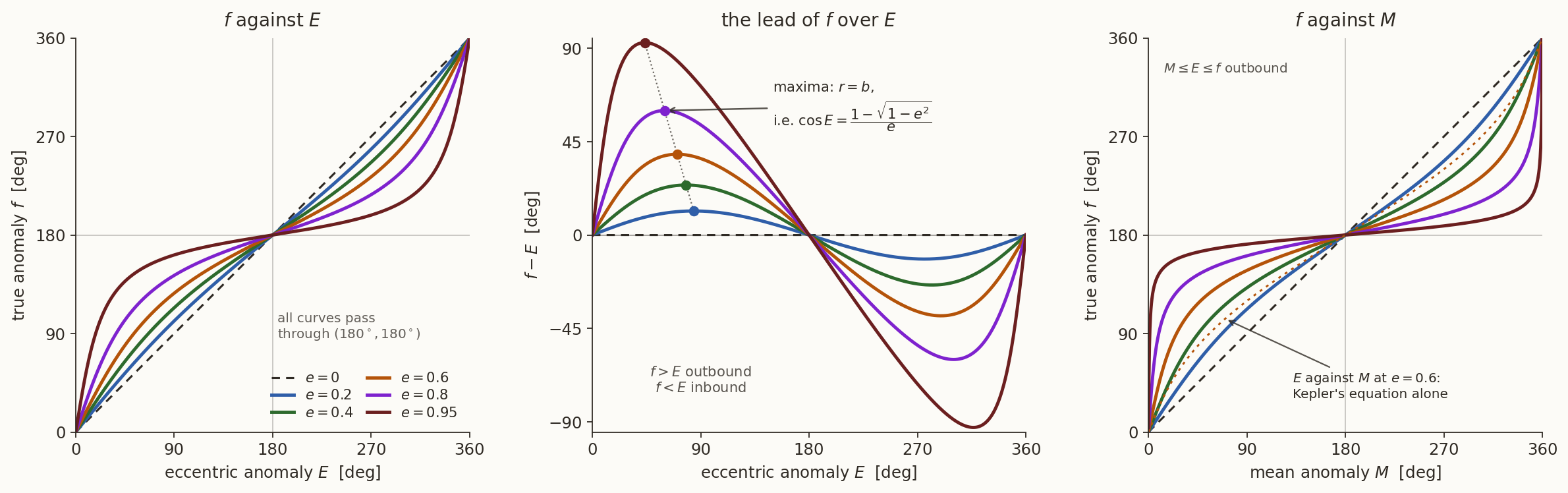
Why the curves bow. Differentiate the half-angle relation \(\tan\frac{f}{2} = \sqrt{\frac{1+e}{1-e}}\,\tan\frac{E}{2}\) and simplify with \(1 + \cos f = \dfrac{(1-e)(1 + \cos E)}{1 - e\cos E}\):
\[
\frac{df}{dE} = \frac{\sqrt{1 - e^{2}}}{1 - e\cos E}
= \frac{b/a}{r/a}
\qquad\Longrightarrow\qquad
\boxed{\;\frac{df}{dE} = \frac{b}{r}\;}
\]
A remarkably clean statement, and it reads off the whole figure:
- \(r < b\) (near periapsis): \(f\) outruns \(E\). The focus is offset towards periapsis, so a small displacement there subtends a large angle at the focus but only a small one at the centre.
- \(r > b\) (near apoapsis): \(f\) falls behind \(E\).
- \(r = b\): the two run level, \(df/dE = 1\), which is exactly the stationary point of \(f - E\) marked on the right-hand panel. Setting \(1 - e\cos E = \sqrt{1-e^{2}}\) gives its location in closed form,
\[
\cos E = \frac{1 - \sqrt{1 - e^{2}}}{e} .
\]
- \(E = 0, \pi\) are fixed points for every \(e\): at the apsides the centre, the focus and the body are collinear, so all three anomalies coincide. This is why the curves in the left panel form a pencil through \((180^{\circ}, 180^{\circ})\).
Two limits worth remembering. For small \(e\),
\[
f = E + e\sin E + O\!\left(e^{2}\right),
\qquad
E = M + e\sin M + O\!\left(e^{2}\right)
\;\Longrightarrow\;
f = M + 2e\sin M + O\!\left(e^{2}\right),
\]
the last being the equation of the centre — for the Earth (\(e = 0.0167\)) it peaks at about \(1.9^{\circ}\) (\(\approx 2e\) radians), and is one of the two terms that make up the equation of time — the other coming from the obliquity of the ecliptic, which is in fact slightly the larger of the two. As \(e \to 1\) the map degenerates towards a step: essentially the whole sweep in \(f\) happens in a vanishing neighbourhood of \(E = 0\), since \(b/r \to \infty\) at periapsis. That is the same stiffness that makes Newton’s method on Kepler’s equation delicate for near-parabolic orbits.
The rotating basis \((\hat{\mathbf{r}}, \hat{\boldsymbol{\theta}})\)
Everything in the velocity derivation rested on two little formulae:
\[
\dot{\hat{\mathbf{r}}} = \dot f\,\hat{\boldsymbol{\theta}}, \qquad
\dot{\hat{\boldsymbol{\theta}}} = -\dot f\,\hat{\mathbf{r}} .
\]
They are worth proving twice — once with components, once without.
Setup. Let \(\hat{\mathbf{P}}\) point from the focus towards periapsis and \(\hat{\mathbf{Q}} = \hat{\mathbf{h}} \times \hat{\mathbf{P}}\) complete a right-handed pair in the orbital plane (the perifocal basis). Both are built from the constants \(\mathbf{e}\) and \(\mathbf{h}\), so both are fixed in space: \(\dot{\hat{\mathbf{P}}} = \dot{\hat{\mathbf{Q}}} = \mathbf{0}\).
Since \(f\) is measured from periapsis,
\[
\hat{\mathbf{r}} = \cos f\,\hat{\mathbf{P}} + \sin f\,\hat{\mathbf{Q}},
\qquad
\hat{\boldsymbol{\theta}} = -\sin f\,\hat{\mathbf{P}} + \cos f\,\hat{\mathbf{Q}} .
\]
Proof 1 — differentiate the components
Only \(f\) depends on time, so the chain rule acts on the sines and cosines alone:
\[
\dot{\hat{\mathbf{r}}}
= \frac{d}{dt}\left(\cos f\,\hat{\mathbf{P}} + \sin f\,\hat{\mathbf{Q}}\right)
= \dot f\left(-\sin f\,\hat{\mathbf{P}} + \cos f\,\hat{\mathbf{Q}}\right)
= \dot f\,\hat{\boldsymbol{\theta}} .
\]
\[
\dot{\hat{\boldsymbol{\theta}}}
= \dot f\left(-\cos f\,\hat{\mathbf{P}} - \sin f\,\hat{\mathbf{Q}}\right)
= -\dot f\,\hat{\mathbf{r}} .
\]
That is the whole proof — but it hides why it is true, so here is the same statement with no components at all.