End-Semester Examination, December 2025

Course	Spaceflight Mechanics (AE313 / AE613), Aerospace Engineering, IIST
Examination	End-Semester, 8 December 2025, 01:30 PM to 04:30 PM, venue D4
Maximum marks	50
Q1	21 marks
Q2	5 marks
Q3	6 marks
Q4	6 marks
Q5	6 marks
Q6	6 marks

Instructions

1. All questions are compulsory.
2. Clearly state all the assumptions/approximations in the derivations/answers.
3. Diagrams and write-up that are not legible will not be graded.
4. All students are allowed two pages of handwritten formula sheet in the exam.

The questions are reproduced as they were set, with their marks. Added for this page: the table of marks above, the folded solution under each question, and the figures of the solutions. Two typographical points: in Q1 the blanks keep the labels they had in the paper, so (i) comes after (m), and a missing opening bracket in (i) has been put back. The paper gave no value of \(\mu_\oplus\); the solutions use \(\mu_\oplus=398\,600\ \mathrm{km^3\,s^{-2}}\) (\(=3.986\times10^{5}\)). With the more exact \(398\,600.4418\) every quoted result is unchanged, except that the circular speed at 7000 km, \(7.5460\) km/s, becomes \(7.5461\) in the last digit. The numbers were checked by endsem-2025-verify.py, which also checks the supporting numbers quoted in the Q1 and Q5 solutions; the verbal answers of Q1 (blanks (e), (f), (g), (o), (q), (r), (s)) are explanations, not computed.

Q1 [21 marks]

We resume our review of the course from where we stopped. After studying two-dimensional planetary motion, we extended the analysis to three dimensions. In doing so, we introduced three additional orbital elements \(i\), \(\Omega\), and \(\omega\), called (a) [0.5 marks] ____________, (b) [0.5 marks] ____________, and (c) [0.5 marks] ____________, respectively. A satellite of Earth with (d) [0.5 marks] ____________ (condition written in terms of the orbital elements) has retrograde motion.

We then studied orbital maneuvers, focusing on impulsive maneuvers rather than continuous-thrust models to simplify the analysis. This was justified by the argument that (e) [2 marks] ________________________.

We showed that (f) [1 mark] ________ (number) transfer orbits exist for transferring a satellite from one elliptical orbit to another. An external criteria was used to choose a particular orbit. The most important criteria we found to be minimization of fuel consumption. This is equivalent to minimizing the total \(\Delta v\) of the transfer. We found that it is always advantageous to perform impulsive maneuvers at the perigee of the first orbit. A heuristic argument in support of this statement is: (g) [2 marks] ________________________.

We also observed that the difference in total mechanical energy \(\left(\tfrac12v^2-\tfrac{\mu}{r}\right)\) between the initial and final orbits does not, by itself, determine the \(\Delta v\) required for transfer. An example of two planar orbits with the same total mechanical energy but a nonzero \(\Delta v\) required for transfer is: (h) [1 mark] __________________.

Next, we explored rendezvous and chase maneuvers between two satellites. We consider a fixed transfer time maneuver. Let the initial state vectors of the chaser and target satellites be \((\mathbf r_c,\mathbf v_c)\) and \((\mathbf r_t,\mathbf v_t)\), respectively. We first determine the position of the target at the rendezvous time. The target state at rendezvous, \((\mathbf r^+_t,\mathbf v^+_t)\), is obtained by solving (j) [1 mark] ____________ equations (name of the equations is expected) for the elliptical and parabolic cases. The chaser state at rendezvous, \((\mathbf r^+_c,\mathbf v^+_c)\), is then found by noting that (k) [1 mark] ____________ for a rendezvous, while (l) [1 mark] ____________ for a chase maneuver. Once the terminal states of both target and chaser are known, we solve (m) [1 mark] ____________ to determine the transfer orbit.

We also studied orbit transfers in 3D. To change the inclination of a satellite by \(45^\circ\) (while keeping all other orbital parameters fixed), we apply a \(\Delta v\) of (i) [1 mark] ____________ at the ascending node.

We then considered interplanetary transfers. To avoid the full multi-body problem, we introduced the concept of the sphere of influence (SOI) for each body. These two ideas require further clarification.

As an example, consider a spacecraft moving under the gravitational attraction of both Earth and Sun. Using Newton’s law of gravitation, we can write the equations of motion of the spacecraft as (n) [2 marks] ________________________. These equations can be integrated numerically (e.g. by RK4) to obtain the trajectory for given initial conditions. With modern computational resources (unlike during the Apollo era), solving these equations is quite feasible. Nevertheless, we still prefer to work with the two-body problem instead of the full multi-body problem because (o) [1 mark] __________________.

Next, we examined the sphere of influence more carefully. The gravitational force due to the Sun is smaller than that due to Earth for any point with \(r<r_{\rm SOI}\), where \(r_{\rm SOI}\) is the radius of Earth’s sphere of influence. (p) [1 mark] True / False ________.

Finally, we returned to Earth-bound ballistic trajectories. We assumed (q) [1 mark] __________________ to make the ballistic trajectories symmetric. In ballistic trajectory problems, we are typically given the launch site, the target site, and the missile velocity at burnout altitude, and are asked to determine (r) [1 mark] __________________.

This completes our brief tour of the course. To conclude, recall that our model of orbital mechanics is a simplified representation of reality. List any four ways in which this model must be modified to better match the real world: (s) [2 marks] ________________________.

Solution to Q1

The blanks keep the labels of the paper. Where a blank has a short answer it is in the table; the longer ones are worked below it.

Blank	Answer	Basis
(a)	inclination	the angle between the orbit plane and the reference (equatorial) plane, that is between \(\mathbf h\) and \(\hat{\mathbf k}\): \(\cos i=h_z/h\)
(b)	right ascension (longitude) of the ascending node	the angle, in the reference plane, from the reference direction (\(\hat{\mathbf i}\), the vernal equinox) to the ascending node
(c)	argument of perigee	the angle, in the orbit plane, from the ascending node to the perigee, in the direction of motion
(d)	\(90^\circ<i\le180^\circ\), that is \(\cos i<0\) or \(h_z<0\)	the satellite then goes round against the Earth’s rotation
(e)	see below	the burn is short compared with the orbit
(f)	infinitely many (\(\infty\))	see below
(g)	see below	the Oberth effect
(h)	see below	the same \(a\), but not the same orbit
(j)	Kepler’s equation (ellipse) and Barker’s equation (parabola)	the time of flight of the target to \(t_f\) gives its true anomaly, and so \((\mathbf r^+_t,\mathbf v^+_t)\); both are forms of the universal Kepler equation
(k)	\(\mathbf r^+_c=\mathbf r^+_t\) and \(\mathbf v^+_c=\mathbf v^+_t\)	rendezvous: same place and same velocity at the meeting time
(l)	\(\mathbf r^+_c=\mathbf r^+_t\) only	chase (intercept): same place, and the velocity is left free
(m)	Lambert’s problem	the orbit joining \(\mathbf r_c\) to \(\mathbf r^+_c=\mathbf r^+_t\) in the given time of flight \(\Delta t\); it gives the two burns
(i)	see below	\(2\,(h/r)\sin22.5^\circ\)
(n)	see below	Newton’s law with two attracting bodies
(o)	see below	closed form against numerical integration
(p)	False	see below
(q)	the burnout and re-entry radii are equal, \(r_{re}=r_{bo}\) (on a spherical, non-rotating Earth)	an ellipse is symmetric about its major axis, so two points at the same distance from the focus are mirror images
(r)	the burnout flight-path angle \(\gamma_{bo}\) (two solutions, a low and a lofted one) and the launch azimuth	\(\gamma_{bo}\) is the one quantity that the guidance system can still choose
(s)	see below	the four omitted forces and effects

(e) The burn lasts a very small fraction of the orbital period, \(t_{\rm burn}/T\ll1\): a chemical stage burns for minutes on an orbit of hours, so the spacecraft hardly moves while it burns. So we replace the burn by an instantaneous change of the velocity at a fixed point, \(\mathbf r^+=\mathbf r^-\) and \(\mathbf v^+=\mathbf v^-+\Delta\mathbf v\), and a transfer becomes a set of two-body conics joined at the burn points. The model fails for an ion engine, which must burn for months and spirals outwards.

(f) Choose any point on the first orbit, any point on the second, and a time of flight: Lambert’s problem gives a conic through them. Each choice gives a different transfer, so there are infinitely many, and an extra criterion (here the least total \(\Delta v\)) is needed to pick one. (If the transfers are restricted to the ones that touch both orbits at their apsides, there are two for coaxial ellipses.)

(g) A burn \(\Delta v\) along the velocity \(v\) changes the specific energy by

\[ \Delta\varepsilon=\tfrac12(v+\Delta v)^2-\tfrac12v^2=v\,\Delta v+\tfrac12\Delta v^2 , \]

so for the same \(\Delta v\) (which by the rocket equation is the same propellant) the energy gained grows with the speed \(v\) at the burn. The speed is largest at the perigee. So the energy needed for the transfer is bought most cheaply there.

(h) A circle of radius \(a\) and an ellipse of semi-major axis \(a\) (say \(e=0.5\)) have the same energy \(-\mu/2a\). They cross where \(r=a\), that is at \(\cos f=-e\) (\(f=120^\circ\)), and there the speeds are equal, because the same energy and the same \(r\) fix the speed. But the velocity directions differ: the ellipse has the flight-path angle \(\gamma=\arcsin e=30^\circ\) and the circle has \(0\). The transfer is a pure rotation of the velocity through \(\gamma\) at constant speed, \(\Delta v=2v\sin(\gamma/2)=2\sqrt{\mu/a}\,\sin15^\circ=0.518\,v_c\). Energy fixes the speed at each radius and not the direction. (Another example: two ellipses of the same \(a\) and \(e\) with their apse lines turned through \(\eta\) need \(\Delta v=2\sqrt{\mu/p}\,e\sin(\eta/2)\).)

(i) A rotation of the orbit through \(\Delta i=45^\circ\) about the line of nodes leaves \(a\), \(e\), \(\Omega\) and \(\omega\) unchanged. At the node the velocity has a part along the line of nodes (the radial speed \(v_r\)) and a part perpendicular to it (the transverse speed \(h/r\)). Only the transverse part is turned,

\[ \Delta v=2\,\frac hr\sin\frac{\Delta i}{2}=2\,v\cos\gamma\,\sin22.5^\circ , \]

where \(\gamma\) is the flight-path angle at the node. For a circular orbit \(\gamma=0\), so \(\Delta v=2\sin22.5^\circ\,v=0.765\,v\) at the speed \(v\) of the orbit.

(n) In an inertial frame, with \(\mathbf r\) the position of the spacecraft and \(\mathbf r_\oplus(t)\), \(\mathbf r_\odot(t)\) those of the Earth and the Sun,

\[ \ddot{\mathbf r}=-\mu_\oplus\frac{\mathbf r-\mathbf r_\oplus}{|\mathbf r-\mathbf r_\oplus|^3}-\mu_\odot\frac{\mathbf r-\mathbf r_\odot}{|\mathbf r-\mathbf r_\odot|^3}. \]

The positions of the two bodies are given functions of time. Relative to the Earth, with \(\mathbf r\) now measured from the Earth and \(\mathbf R\) the position of the Sun relative to the Earth, the Earth’s own acceleration towards the Sun has to be subtracted:

\[ \ddot{\mathbf r}=-\mu_\oplus\frac{\mathbf r}{r^3}-\mu_\odot\Bigl[\frac{\mathbf r-\mathbf R}{|\mathbf r-\mathbf R|^3}+\frac{\mathbf R}{R^3}\Bigr]. \]

The first term is the two-body problem; the bracket is the Sun’s perturbation, which has the “direct” and the “indirect” part.

(o) The two-body problem has a closed-form solution (conics, Kepler’s equation), and so gives formulas, insight and a fast first design. The problem of three or more bodies has no general closed-form solution; it needs numerical integration for every trial trajectory, and its results give little physical insight. Inside the sphere of influence of a body the other attraction is a small perturbation, so a two-body conic is a good approximation of the motion.

(p) False. The Sun does pull harder than the Earth over most of the Earth’s sphere of influence. At \(r_{\rm SOI}=9.25\times10^5\) km the Sun’s pull is \(\mu_\odot/R^2=5.93\times10^{-6}\ \mathrm{km/s^2}\) and the Earth’s is \(\mu_\oplus/r_{\rm SOI}^2=4.66\times10^{-7}\ \mathrm{km/s^2}\): the Sun’s is \(12.7\) times larger. The two are equal at \(r=R\sqrt{\mu_\oplus/\mu_\odot}=2.6\times10^5\) km, \(0.28\,r_{\rm SOI}\), so between \(2.6\times10^5\) km and \(r_{\rm SOI}\) the Sun’s pull is the larger. What matters is not the pull itself but the difference between the Sun’s pull on the spacecraft and on the Earth, because both fall towards the Sun together. That differential (tidal) acceleration is about \(2\mu_\odot r/R^3=7.3\times10^{-8}\ \mathrm{km/s^2}\) at \(r_{\rm SOI}\), \(16\%\) of the Earth’s pull there. The sphere of influence is defined by this ratio of the perturbation to the main acceleration (Laplace’s criterion), not by equal forces.

(s) Any four of: (1) the Earth is not a sphere: its oblateness (\(J_2\)) and higher harmonics make \(\Omega\) and \(\omega\) drift; (2) atmospheric drag, in low orbits and on re-entry; (3) the gravity of other bodies, the Sun and the Moon; (4) solar radiation pressure on large, light spacecraft; (5) burns are not instantaneous: finite thrust causes gravity and steering losses; (6) the Earth rotates (ballistic missiles); (7) relativistic corrections (precise navigation).

Q2 [5 marks]

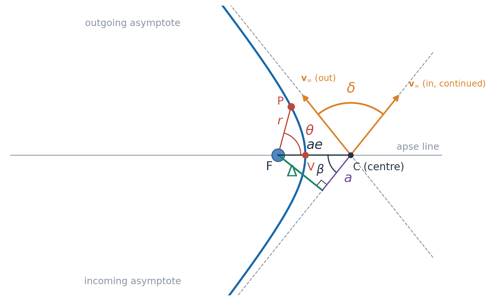
Draw the diagram of a hyperbolic orbit. Show the asymptote, apse line, true anomaly (\(\theta\)), aiming radius (\(\Delta\)) and turn angle (\(\delta\)). Also derive the expression for the aiming radius in terms of \(a\) and \(e\) from geometry.

Solution to Q2

What is to be shown. The aiming radius \(\Delta\) is the perpendicular distance from the focus to the asymptote along which the body arrives: the distance by which it would miss the attracting body if it were not deflected. We have to show \(\Delta=a\sqrt{e^2-1}\) from the geometry of the figure. In this solution \(a\) means the positive number \(|a|\); with the sign convention \(a=-\mu/2\varepsilon<0\) of the course, read \(\Delta=-a\sqrt{e^2-1}\).

Figure 1: A hyperbolic orbit, drawn for \(e=1.6\). F is the focus (the attracting body), V the periapsis, C the centre. The apse line is the line FVC. The two asymptotes cross at C. \(\theta\) is the true anomaly of the point P, measured from the apse line at F. The aiming radius \(\Delta\) is the perpendicular FN from F to the incoming asymptote. The turn angle \(\delta\) is the angle between the incoming velocity at infinity (continued past C) and the outgoing one.

Step 1: the direction of the asymptotes. The orbit is \(r=p/(1+e\cos\theta)\) with \(p=a(e^2-1)\). The body is infinitely far away when the denominator is zero,

\[ 1+e\cos\theta_\infty=0\quad\Longrightarrow\quad\cos\theta_\infty=-\frac1e . \]

The asymptotes are the straight lines in the directions \(\pm\theta_\infty\). Let \(\beta=\pi-\theta_\infty\) be the acute angle that each makes with the apse line: \(\cos\beta=1/e\), so \(\sin\beta=\sqrt{e^2-1}/e\).

Step 2: where the asymptotes cross. The two asymptotes cross at the centre C of the hyperbola, the point halfway between its two vertices, each of which is at the distance \(a\) from C. The periapsis is a vertex, and from the orbit equation its distance from the focus is \(r_p=p/(1+e)=a(e^2-1)/(1+e)=a(e-1)\). So the focus is beyond the vertex, and

\[ FC=r_p+a=a(e-1)+a=ae . \]

Step 3: the triangle F, N, C. Let N be the foot of the perpendicular from F to the incoming asymptote. The triangle FNC is right-angled at N, its hypotenuse is \(FC=ae\), and the angle at C is \(\beta\). The side opposite to \(\beta\) is the aiming radius:

\[ \boxed{\Delta=FC\,\sin\beta=ae\cdot\frac{\sqrt{e^2-1}}{e}=a\sqrt{e^2-1}} \]

As a check, the side next to \(\beta\) is \(CN=FC\cos\beta=ae/e=a\), and Pythagoras gives \(\Delta^2=(ae)^2-a^2=a^2(e^2-1)\), the same.

Step 4: the turn angle. The body arrives moving along the incoming asymptote, which points at the angle \(\pi-\theta_\infty\) from the apse line, and leaves along the outgoing one at \(\theta_\infty\). The velocity turns through

\[ \delta=\theta_\infty-(\pi-\theta_\infty)=2\theta_\infty-\pi=2\arcsin\frac1e,\qquad\text{so}\qquad\sin\frac\delta2=\frac1e . \]

Checks. (i) Physical meaning: the angular momentum is the speed at infinity times the moment arm, \(h=\Delta\,v_\infty\). With \(h=\sqrt{\mu p}\) and \(v_\infty=\sqrt{\mu/a}\) this gives \(\Delta=\sqrt{\mu a(e^2-1)}\big/\sqrt{\mu/a}=a\sqrt{e^2-1}\), the same result. (ii) Limits: for \(e\to1^+\), \(\Delta\to0\) and \(\delta\to180^\circ\) (a head-on fall that goes straight round the body); for \(e\to\infty\), \(\delta\to0\) (a straight line) and \(\Delta\to ae\).

Q3 [6 marks]

Calculate all the six orbital parameters of the satellite given the state vector \(\mathbf r=-6045\,\hat{\mathbf i}-3490\,\hat{\mathbf j}+2500\,\hat{\mathbf k}\) km and \(\mathbf v=-3.457\,\hat{\mathbf i}+6.618\,\hat{\mathbf j}+2.533\,\hat{\mathbf k}\) km/s.

Solution to Q3

Plan. The six elements are \(a\) (or \(h\)), \(e\), \(i\), \(\Omega\), \(\omega\) and \(\theta\). Each one is read from a vector built out of the state: \(\mathbf h=\mathbf r\times\mathbf v\) gives \(h\) and \(i\); the node vector \(\mathbf N=\hat{\mathbf k}\times\mathbf h\) gives \(\Omega\); the eccentricity vector \(\mathbf e\) gives \(e\), then \(\omega\) (with \(\mathbf N\)) and \(\theta\) (with \(\mathbf r\)). An arccosine only gives an angle between \(0^\circ\) and \(180^\circ\), so for \(\Omega\), \(\omega\) and \(\theta\) the half-plane has to be decided from the sign of one component. Take \(\mu_\oplus=398\,600\ \mathrm{km^3/s^2}\).

Step 1: lengths and the radial speed.

\[ r=\sqrt{6045^2+3490^2+2500^2}=7414.3\ \text{km},\qquad v=\sqrt{3.457^2+6.618^2+2.533^2}=7.8845\ \text{km/s}, \]

\[ \mathbf r\cdot\mathbf v=(-6045)(-3.457)+(-3490)(6.618)+(2500)(2.533)=4133.2\ \mathrm{km^2/s},\qquad v_r=\frac{\mathbf r\cdot\mathbf v}{r}=+0.5575\ \text{km/s}. \]

The radial speed is positive: the satellite is moving away from the Earth, so it is between perigee and apogee on the outbound half.

Step 2: angular momentum, \(h\) and \(i\).

\[ \mathbf h=\mathbf r\times\mathbf v=\begin{vmatrix}\hat{\mathbf i}&\hat{\mathbf j}&\hat{\mathbf k}\\-6045&-3490&2500\\-3.457&6.618&2.533\end{vmatrix} =(-25\,385,\ 6669.5,\ -52\,071)\ \mathrm{km^2/s},\qquad h=58\,312\ \mathrm{km^2/s}. \]

\[ \cos i=\frac{h_z}{h}=\frac{-52\,071}{58\,312}=-0.8930\quad\Longrightarrow\quad i=153.25^\circ . \]

There is no ambiguity for \(i\): it lies between \(0^\circ\) and \(180^\circ\), as the arccosine does. Since \(i>90^\circ\) the orbit is retrograde (see Q1(d)).

Step 3: the node, \(\Omega\). The line of nodes points along \(\mathbf N=\hat{\mathbf k}\times\mathbf h=(-h_y,\ h_x,\ 0)=(-6669.5,\ -25\,385,\ 0)\), with \(N=26\,247\) km\(^2\)/s. Then

\[ \cos\Omega=\frac{N_x}{N}=-0.2541\ \Rightarrow\ \arccos=104.72^\circ . \]

The test is the sign of \(N_y\): here \(N_y<0\), so the node is in the lower half-plane and \(\Omega=360^\circ-104.72^\circ=\mathbf{255.28^\circ}\).

Step 4: the eccentricity vector, \(e\). From \(\mathbf e=\dfrac1\mu\left[\left(v^2-\dfrac\mu r\right)\mathbf r-(\mathbf r\cdot\mathbf v)\,\mathbf v\right]\), with \(v^2-\mu/r=62.165-53.761=8.404\ \mathrm{km^2/s^2}\),

\[ \mathbf e=\frac{1}{398\,600}\Bigl[8.404\,(-6045,\,-3490,\,2500)-4133.2\,(-3.457,\,6.618,\,2.533)\Bigr]=(-0.0916,\ -0.1422,\ 0.0264), \]

so \(e=|\mathbf e|=\mathbf{0.1712}\). This is less than \(1\): an ellipse.

Step 5: the argument of perigee, \(\omega\).

\[ \cos\omega=\frac{\mathbf N\cdot\mathbf e}{N\,e}=0.9393\ \Rightarrow\ \arccos=20.07^\circ , \]

and the test is the sign of \(e_z\): \(e_z=+0.0264>0\), so the perigee is north of the equator, \(\omega<180^\circ\) and \(\omega=\mathbf{20.07^\circ}\).

Step 6: the true anomaly, \(\theta\).

\[ \cos\theta=\frac{\mathbf e\cdot\mathbf r}{e\,r}=0.8793\ \Rightarrow\ \arccos=28.45^\circ , \]

and the test is the sign of \(v_r\): \(v_r>0\), so \(\theta<180^\circ\) and \(\theta=\mathbf{28.45^\circ}\).

Step 7: the semi-major axis. \(a=\dfrac{h^2}{\mu(1-e^2)}=\dfrac{58\,312^2}{398\,600\,(1-0.1712^2)}=\mathbf{8788\ km}\).

\(a\)	\(e\)	\(i\)	\(\Omega\)	\(\omega\)	\(\theta\)
\(8788\) km (or \(h=58\,312\) km\(^2\)/s)	\(0.1712\)	\(153.25^\circ\)	\(255.28^\circ\)	\(20.07^\circ\)	\(28.45^\circ\)

Checks. \(r_p=a(1-e)=7283\) km and \(r_a=a(1+e)=10\,293\) km: the radius \(7414\) km lies between them, and just above the perigee, as \(\theta=28^\circ\) and \(v_r>0\) say. The specific energy is \(v^2/2-\mu/r=-22.68\ \mathrm{km^2/s^2}=-\mu/2a\), the period is \(2\pi\sqrt{a^3/\mu}=2.28\) h.

Q4 [6 marks]

A spacecraft at a radius \(r\) has a speed \(v\) and a flight path angle \(\gamma\). What is \(\sigma\) in the following expression in terms of \(r\), \(v\) and \(\gamma\).

\[ e=\sqrt{1+\sigma(\sigma-2)\cos^2\gamma} \]

Solution to Q4

What is to be shown. We know \(r\), \(v\) and \(\gamma\) at one point, so we can find the energy and the angular momentum there, and the eccentricity follows from those two. Then we compare the result with the given form to read off \(\sigma\).

Step 1: the energy and the angular momentum. The flight-path angle \(\gamma\) is measured from the local horizontal, so the transverse component of the velocity is \(v\cos\gamma\):

\[ \varepsilon=\frac{v^2}{2}-\frac{\mu}{r},\qquad h=r\,v_\perp=r\,v\cos\gamma . \]

Step 2: \(e\) from \(\varepsilon\) and \(h\). For any conic \(p=h^2/\mu\) and \(p=a(1-e^2)\) with \(a=-\mu/(2\varepsilon)\). Hence

\[ 1-e^2=\frac pa=\frac{h^2}{\mu}\cdot\Bigl(-\frac{2\varepsilon}{\mu}\Bigr) \quad\Longrightarrow\quad e^2=1+\frac{2\varepsilon h^2}{\mu^2}. \]

Step 3: substitute.

\[ e^2=1+\frac{2}{\mu^2}\Bigl(\frac{v^2}{2}-\frac\mu r\Bigr)r^2v^2\cos^2\gamma =1+\frac{(v^2-2\mu/r)\,r^2v^2}{\mu^2}\cos^2\gamma . \]

To bring this to the form \(\sigma(\sigma-2)\), write the factor in front of \(\cos^2\gamma\) as a product of two things in \(\mu/r\) and \(v^2\). Divide and multiply by \(\mu/r\) twice:

\[ \frac{(v^2-2\mu/r)\,r^2v^2}{\mu^2}=\frac{r v^2}{\mu}\cdot\frac{r\,(v^2-2\mu/r)}{\mu}=\frac{rv^2}{\mu}\Bigl(\frac{rv^2}{\mu}-2\Bigr). \]

So with

\[ \boxed{\sigma=\frac{r\,v^2}{\mu}=\frac{v^2}{v_c^2}}\qquad\bigl(v_c=\sqrt{\mu/r}\ \text{the local circular speed}\bigr) \]

we get exactly \(e^2=1+\sigma(\sigma-2)\cos^2\gamma\).

Physical reading and checks. \(\sigma\) is the square of the speed measured in units of the local circular speed. (i) A circular orbit has \(v=v_c\) and \(\gamma=0\), so \(\sigma=1\) and \(e=\sqrt{1+(1)(-1)}=0\). (ii) The escape speed is \(v=\sqrt2\,v_c\), so \(\sigma=2\) and \(e=1\) for every \(\gamma\): a parabola, whatever the direction of the velocity. (iii) At an apse, \(\gamma=0\), and \(e=|\sigma-1|\), so a speed \(v>v_c\) at an apse is the perigee, and \(v<v_c\) is the apogee. (iv) \(\sigma(\sigma-2)<0\) for \(0<\sigma<2\): those are the ellipses, and \(\sigma>2\) gives the hyperbolas. (In Bate’s treatment of ballistic flight, this \(\sigma\) is called \(Q\).)

Q5 [6 marks]

Find the total \(\Delta v\) requirement for bielliptic Hohmann transfer from a geocentric circular orbit of 7000 km radius to one of 105,000 km radius. Let the apogee of the first ellipse be 210,000 km. Compare the \(\Delta v\) schedule and total flight time with that for an ordinary single Hohmann transfer ellipse.

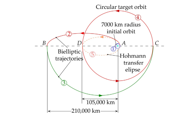
Figure 2: The question’s figure. A: the 7000 km initial orbit; the bielliptic transfer is the arcs 2 and 3 with the burns at A, B and C; the circular target orbit is the arc 4 and the single Hohmann ellipse is the dashed arc 5.

Solution to Q5

What is to be found. The three burns of the bi-elliptic transfer, their sum and the time it takes; the two burns of the Hohmann transfer between the same circles; and the comparison. Take \(\mu_\oplus=398\,600\ \mathrm{km^3/s^2}\).

The orbits. Using the labels of the figure, the points A, B and C are on the line of apsides. A is the point on the 7000 km circle where the first burn is made; B is the apogee of the first ellipse; C is the point of the 105,000 km circle where the second ellipse ends. Every burn is at an apse, and so is tangential, and each \(\Delta v\) is the difference of two speeds, both found from the vis-viva equation \(v^2=\mu(2/r-1/a)\).

orbit	from	to	\(r_p\) [km]	\(r_a\) [km]	\(a\) [km]
circle \(1\) (initial)			\(7000\)	\(7000\)	\(7000\)
ellipse I	A	B	\(7000\)	\(210\,000\)	\(108\,500\)
ellipse II	B	C	\(105\,000\)	\(210\,000\)	\(157\,500\)
circle \(2\) (target)			\(105\,000\)	\(105\,000\)	\(105\,000\)
Hohmann ellipse H	A	D	\(7000\)	\(105\,000\)	\(56\,000\)

Step 1: the speeds. The circular speeds are \(v_{c1}=\sqrt{\mu/7000}=7.5460\) km/s and \(v_{c2}=\sqrt{\mu/105\,000}=1.9484\) km/s. On the ellipses:

\[ \begin{aligned} v_{A,\rm I}&=\sqrt{\mu\Bigl(\tfrac2{7000}-\tfrac1{108\,500}\Bigr)}=10.4982\ \text{km/s}, & v_{B,\rm I}&=\sqrt{\mu\Bigl(\tfrac2{210\,000}-\tfrac1{108\,500}\Bigr)}=0.3499\ \text{km/s},\\ v_{B,\rm II}&=\sqrt{\mu\Bigl(\tfrac2{210\,000}-\tfrac1{157\,500}\Bigr)}=1.1249\ \text{km/s}, & v_{C,\rm II}&=\sqrt{\mu\Bigl(\tfrac2{105\,000}-\tfrac1{157\,500}\Bigr)}=2.2498\ \text{km/s}. \end{aligned} \]

Step 2: the burns.

burn	where	speed before	speed after	\(\Delta v\) [km/s]	direction
1	A	\(7.5460\)	\(10.4982\)	\(2.9521\)	prograde
2	B	\(0.3499\)	\(1.1249\)	\(0.7750\)	prograde
3	C	\(2.2498\)	\(1.9484\)	\(0.3014\)	retrograde

The third burn is a brake: ellipse II arrives at C, its perigee, faster than the circular speed of the target orbit. The total is \(\Delta v_{\rm bi}=2.9521+0.7750+0.3014=\mathbf{4.0285}\) km/s.

Step 3: the flight time. Each transfer ellipse is flown for half a period, \(t=\pi\sqrt{a^3/\mu}\):

\[ t_{\rm I}=\pi\sqrt{\frac{108\,500^3}{398\,600}}=49.40\ \text{h},\qquad t_{\rm II}=\pi\sqrt{\frac{157\,500^3}{398\,600}}=86.40\ \text{h},\qquad t_{\rm bi}=135.80\ \text{h}=5.66\ \text{days}. \]

Step 4: the Hohmann transfer. On ellipse H, \(v_{A,\rm H}=\sqrt{\mu(2/7000-1/56\,000)}=10.3329\) km/s and \(v_{D,\rm H}=\sqrt{\mu(2/105\,000-1/56\,000)}=0.6889\) km/s, so

\[ \Delta v_A=10.3329-7.5460=2.7868\ \text{km/s},\qquad \Delta v_D=1.9484-0.6889=1.2595\ \text{km/s}, \]

both prograde, a total \(\Delta v_{\rm H}=\mathbf{4.0463}\) km/s, flown in \(t_{\rm H}=\pi\sqrt{56\,000^3/\mu}=\mathbf{18.32}\) h.

Step 5: the comparison.

	first burn	second burn	third burn	total \(\Delta v\)	flight time
Hohmann	\(2.7868\) (A)	\(1.2595\) (D)	none	\(4.0463\) km/s	\(18.32\) h
bi-elliptic	\(2.9521\) (A)	\(0.7750\) (B)	\(0.3014\) (C)	\(4.0285\) km/s	\(135.80\) h

The bi-elliptic transfer saves \(17.8\) m/s, \(0.44\%\) of the \(\Delta v\), and takes \(7.4\) times as long. Its first burn is \(0.165\) km/s larger (it throws the vehicle much higher), but it then changes the perigee from \(7000\) km to \(105\,000\) km at B, where the speed is only \(0.35\) km/s and the burn is cheap, and the arrival brake is small (\(0.301\) against \(1.260\) km/s). The saving is real but small, and it is bought with days of flight.

When does the bi-elliptic transfer win? The ratio of the radii is \(R=r_C/r_A=15\). A bi-elliptic transfer can beat the Hohmann one for \(R>11.94\); for \(R>15.58\) it always does, for any apogee beyond the target orbit; between the two thresholds, as here, it wins only if its apogee is high enough. For \(R=15\) the break-even apogee is \(127\,300\) km (\(18.2\,r_A\)), so the given \(210\,000\) km (\(30\,r_A\)) wins. The higher the apogee, the larger the saving, and the longer the flight.

Q6 [6 marks]

During the test firing of a ballistic missile, the following measurements were made: \(h_{bo}\) = 1/5 DU, \(v_{bo}\) = 2/3 DU/TU, \(h_{apogee}\) = 0.5 DU. Assuming a symmetrical trajectory, what was the free-flight range of the missile during this test? (1 DU = 6378 km, 1 DU/TU = 7.905 km/s)

Solution to Q6

What is to be found. The free flight is a piece of a Kepler ellipse. A symmetrical trajectory has the same radius at burnout and at re-entry, so it is symmetric about the apse line and the range angle follows from the true anomaly at burnout. In this question \(h_{bo}\) and \(h_{apogee}\) are altitudes above the surface (not angular momentum). In the canonical units \(\mu_\oplus=1\ \mathrm{DU^3/TU^2}\) and the radius of the Earth is \(1\) DU, so the radii from the centre are

\[ r_{bo}=1+\tfrac15=1.2\ \text{DU},\qquad r_a=1+0.5=1.5\ \text{DU},\qquad v_{bo}=\tfrac23\ \text{DU/TU}. \]

Step 1: the ellipse from the energy and the apogee. The energy at burnout, with \(\mu=1\), is

\[ \varepsilon=\frac{v_{bo}^2}{2}-\frac{\mu}{r_{bo}}=\frac{4/9}{2}-\frac1{1.2}=-0.6111\ \frac{\mathrm{DU^2}}{\mathrm{TU^2}},\qquad a=-\frac{\mu}{2\varepsilon}=\frac{1}{1.2222}=\frac{9}{11}=0.8182\ \text{DU}. \]

The apogee is \(r_a=a(1+e)\), so

\[ e=\frac{r_a}{a}-1=\frac{1.5}{9/11}-1=\frac56=0.8333,\qquad p=a(1-e^2)=\frac9{11}\cdot\frac{11}{36}=\frac14\ \text{DU}. \]

(The perigee is at \(r_p=a(1-e)=0.136\) DU, inside the Earth, as it is for a missile: the flight is only the arc above the surface.)

Step 2: the true anomaly at burnout. From the orbit equation at \(r=r_{bo}\),

\[ r_{bo}=\frac{p}{1+e\cos f_{bo}}\ \Longrightarrow\ \cos f_{bo}=\frac1e\Bigl(\frac{p}{r_{bo}}-1\Bigr)=\frac65\Bigl(\frac{0.25}{1.2}-1\Bigr)=-0.95, \qquad f_{bo}=161.81^\circ . \]

The vehicle is on the outbound branch, \(f_{bo}\) between \(90^\circ\) and \(180^\circ\) and just before the apogee at \(180^\circ\).

Step 3: the range angle. A symmetric trajectory is mirror-symmetric about the apse line: it reaches the same radius again at the true anomaly \(360^\circ-f_{bo}\), so it sweeps the angle

\[ \psi=2\,(180^\circ-f_{bo})=2\,(18.19^\circ)=36.39^\circ=0.6351\ \text{rad}. \]

Step 4: the range. The range on the surface is the arc of the Earth’s circle under the angle \(\psi\) at the centre,

\[ \text{range}=R_\oplus\,\psi=0.6351\ \text{DU}\times6378\ \text{km/DU}=\mathbf{4051\ km}. \]

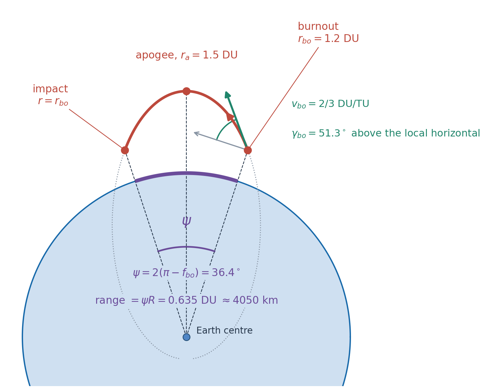
Figure 3: The free flight of Q6: the arc of the ellipse above the Earth’s surface, from burnout (right) through the apogee to impact (left). The ellipse is \(a=9/11\) DU, \(e=5/6\); its perigee is inside the Earth (dotted). The range is the arc of the Earth’s surface under the angle \(\psi\). At burnout the grey arrow is the local horizontal and the green arrow the velocity, which is raised by \(\gamma_{bo}\) above it.

Checks. (i) The units: \(1\ \mathrm{DU/TU}=\sqrt{\mu/R}=7.905\) km/s, so \(v_{bo}=5.27\) km/s, and the apogee altitude is \(0.5\times6378=3189\) km. (ii) Against Q4: the burnout value of \(\sigma\) is \(Q=r_{bo}v_{bo}^2/\mu=0.5333\), and \(e^2=1+Q(Q-2)\cos^2\gamma_{bo}\) gives \(\cos^2\gamma_{bo}=0.3906\), \(\gamma_{bo}=51.3^\circ\): a lofted flight. The range equation \(\tan(\psi/2)=\dfrac{Q\sin\gamma\cos\gamma}{1-Q\cos^2\gamma}=0.3287\) then gives \(\psi=36.39^\circ\) again. (iii) Numerical integration of the two-body motion from the burnout state, with \(\gamma_{bo}=51.3^\circ\), returns to \(r=1.2\) DU after \(36.39^\circ\) and reaches an apogee of \(1.5000\) DU. (iv) The flight time, from Kepler’s equation, is \(2.467\) TU \(=33.2\) min (\(1\) TU \(=806.8\) s).